Topology Optimization with a Poisson Equation

Solving topology optimization problems with a level-set method

The general form of a topology optimization problem is given by

\[ \min_\Omega J(\Omega), \]

i.e., we want to minimize some cost functional \(J\) depending on a geometry or set \(\Omega\) which is contained in some hold-all domain \(\mathrm{D}\) by varying the topology and shape of \(\Omega\). In contrast to shape optimization problems we have discussed previously, topology optimization considers topological changes of \(\Omega\), i.e., the addition or removal of material.

One can represent the domain \(\Omega\) with a continuous level-set function \(\Psi \colon \mathrm{D} \to \mathbb{R}\) as follows:

\[\begin{split} \begin{align} \Psi(x) < 0 \quad &\Leftrightarrow \quad x \in \Omega,\\ \Psi(x) > 0 \quad &\Leftrightarrow \quad x \in \mathcal{D} \setminus \bar{\Omega},\\ \Psi(x) = 0 \quad &\Leftrightarrow \quad x \in \partial \Omega \setminus \partial \mathrm{D}. \end{align} \end{split}\]

Assuming that the topological derivative of the problem exists, which we denote by \(DJ(\Omega)\), then the generalized topological derivative is given by

\[\begin{split} \mathcal{D}J(\Omega)(x) = \begin{cases} -DJ(\Omega)(x) \quad &\text{ if } x \in \Omega,\\ DJ(\Omega)(x) \quad &\text{ if } x \in \mathcal{D} \setminus \bar{\Omega}. \end{cases} \end{split}\]

This is motivated by the fact that if there exists some constant \(c > 0\) such that

\[ \mathcal{D}J(\Omega)(x) = c\Psi(x) \quad \text{ for all } x \in \mathrm{D}, \]

then we have that \(DJ(\Omega) \geq 0\) which is a necessary condition for \(\Omega\) being a local minimizer of the problem. According to this, several optimization algorithms have been developed in the literature to solve topology optimization problems with level-set methods. We refer the reader to Blauth and Sturm - Quasi-Newton methods for topology optimization using a level-set method for a detailed discussion of the algorithms implemented in cashocs.

Problem Formulation

In this demo, we investigate the basics of using cashocs for solving topology optimization problems with a level-set approach. This approachs goes back to Amstutz and Andrä - A new algorithm for topology optimization using a level-set method and in cashocs we have implemented novel gradient-type and quasi-Newton methods for solving such problems from Blauth and Sturm - Quasi-Newton methods for topology optimization using a level-set method.

In this demo, we consider the following model problem

\[\begin{split} \begin{align} &\min_{\Omega,u} J(\Omega, u) = \frac{1}{2} \int_\mathrm{D} \left( u - u_\mathrm{des} \right)^2 \text{ d}x\\ &\text{subject to} \qquad \begin{alignedat}[t]{2} - \Delta u + \alpha_\Omega u &= f_\Omega \quad &&\text{ in } \mathrm{D},\\ u &= 0 \quad &&\text{ on } \partial \mathrm{D}. \end{alignedat} \end{align} \end{split}\]

Here, \(\alpha_\Omega\) and \(f_\Omega\) have jumps between \(\Omega\) and \(\mathrm{D} \setminus \bar{\Omega}\) and are given by \(\alpha_\Omega(x) = \chi_\Omega(x)\alpha_\mathrm{in} + \chi_{\Omega^c}(x) \alpha_\mathrm{out}\) and \(f_\Omega(x) = \chi_\Omega(x) f_\mathrm{in} + \chi_{\Omega^c}(x) f_\mathrm{out}\) with \(\alpha_\mathrm{in}, \alpha_\mathrm{out} > 0\) and \(f_\mathrm{in}, f_\mathrm{out} \in \mathbb{R}\), and \(\Omega^c = \mathrm{D} \setminus \bar{\Omega}\) is the complement of \(\Omega\) in \(\mathrm{D}\). Moreover, \(u_\mathrm{des}\) is a desired state, which in our case comes from the solution of the state equation for a desired shape, which we want to recover by the above problem. The generalized topological derivative for this problem is given by

\[ \mathcal{D}J(\Omega)(x) = (\alpha_\mathrm{in} - \alpha_\mathrm{out}) u(x)p(x) - (f_\mathrm{in} - f_\mathrm{out})p(x), \]

where \(u\) solves the state equation and \(p\) solves the adjoint equation.

Attention

There is a typo in our paper Blauth and Sturm - Quasi-Newton methods for topology optimization using a level-set method, i.e., in the paper a minus sign is missing. The topological derivative as stated here is, in fact, correct.

Implementation

The complete python code can be found in the file demo_poisson_clover.py, and the corresponding config can be found in config.ini.

Initialization and setup

As usual, we start by using a wildcard import for FEniCS and by importing cashocs

from fenics import *

import cashocs

Next, as before, we can specify the verbosity of cashocs with the line

cashocs.set_log_level(cashocs.LogLevel.INFO)

As with the other problem types, the solution algorithms of cashocs can be adapted with the help of configuration files, which is loaded with the load_config function

cfg = cashocs.load_config("config.ini")

In the next step, we define the mesh used for discretization of the hold-all domain \(\mathrm{D}\). To do so, we use the built-in regular_box_mesh function, which gives us a discretization of \(\mathrm{D} = (-2, 2)^2\).

mesh, subdomains, boundaries, dx, ds, dS = cashocs.regular_box_mesh(
    n=32, start_x=-2, start_y=-2, end_x=2, end_y=2, diagonal="crossed"
)

Now, we define the function spaces required for solving the state system, i.e., a finite element space consisting of piecewise linear Lagrange elements, and we define a finite element space consisting of piecewise constant elements, which is used to discretize the jumping coefficients \(\alpha_\Omega\) and \(f_\Omega\).

V = FunctionSpace(mesh, "CG", 1)
DG0 = FunctionSpace(mesh, "DG", 0)

Now, we define the level-set function used to represent our domain \(\Omega\) and initialize \(\Omega\) to the empty set by setting \(\Psi = 1\) with the lines

psi = Function(V)
psi.vector().vec().set(1.0)
psi.vector().apply("")

Definition of the Jumping Coefficients

We define the constants for the jumping coefficients as follows

alpha_in = 10.0
alpha_out = 1.0
alpha = Function(DG0)

f_in = 10.0
f_out = 1.0
f = Function(DG0)

Note

As the jumping coefficients \(\alpha\) and \(f\) are piecewise constant for each part of the considered domain, it is natural to represent them using piecewise constant (in each mesh cell) functions from a discontinuous Lagrange FEM function space. This approach is also mandatory for topology optimization. Note that cells, which are “cut” by the level-set function, an average of the coefficients will be computed, as detailed later.

Computation of the Desired State

Next, we define the desired state \(u_\mathrm{des}\) for our problem by solving the state system for a prescribed desired shape. This is done in the following function. We first state the code below and then go over the function in more details.

def create_desired_state():
    a = 4.0 / 5.0
    b = 2

    f_expr = Expression(
        "0.1 * ( "
        + "(sqrt(pow(x[0] - a, 2) + b * pow(x[1], 2)) - 1)"
        + "* (sqrt(pow(x[0] + a, 2) + b * pow(x[1], 2)) - 1)"
        + "* (sqrt(b * pow(x[0], 2) + pow(x[1] - a, 2)) - 1)"
        + "* (sqrt(b * pow(x[0], 2) + pow(x[1] + a, 2)) - 1)"
        + "- 0.001)",
        degree=1,
        a=a,
        b=b,
    )
    psi_des = interpolate(f_expr, V)

    cashocs.interpolate_levelset_function_to_cells(psi_des, alpha_in, alpha_out, alpha)
    cashocs.interpolate_levelset_function_to_cells(psi_des, f_in, f_out, f)

    y_des = Function(V)
    v = TestFunction(V)

    F = dot(grad(y_des), grad(v)) * dx + alpha * y_des * v * dx - f * v * dx
    bcs = cashocs.create_dirichlet_bcs(V, Constant(0.0), boundaries, [1, 2, 3, 4])

    cashocs.newton_solve(F, y_des, bcs, is_linear=True)

    return y_des, psi_des

Descripion of the define_desired_state function

The above code starts with defining a level-set function based on a clover-type shape, hence the name of this demo, which is done with the lines

a = 4.0 / 5.0
b = 2

f_expr = Expression(
    "0.1 * ( "
    + "(sqrt(pow(x[0] - a, 2) + b * pow(x[1], 2)) - 1)"
    + "* (sqrt(pow(x[0] + a, 2) + b * pow(x[1], 2)) - 1)"
    + "* (sqrt(b * pow(x[0], 2) + pow(x[1] - a, 2)) - 1)"
    + "* (sqrt(b * pow(x[0], 2) + pow(x[1] + a, 2)) - 1)"
    + "- 0.001)",
    degree=1,
    a=a,
    b=b,
)
psi_des = interpolate(f_expr, V)

Note, that this level-set function is taken from the NGSolve Tutorials

Then, the values of the jumping coefficients \(\alpha\) and \(f\) are computed for this level-set function, using the interpolate_levelset_function_to_cells, which sets the piecewise constant functions alpha and f to the appropriate values according to the level-set function:

cashocs.interpolate_levelset_function_to_cells(psi_des, alpha_in, alpha_out, alpha)
cashocs.interpolate_levelset_function_to_cells(psi_des, f_in, f_out, f)

Finally, the state system corresponding to the desired shape is written out and solved with cashocs using the lines

y_des = Function(V)
v = TestFunction(V)

F = dot(grad(y_des), grad(v)) * dx + alpha * y_des * v * dx - f * v * dx
bcs = cashocs.create_dirichlet_bcs(V, Constant(0.0), boundaries, [1, 2, 3, 4])

cashocs.newton_solve(F, y_des, bcs, is_linear=True)

return y_des, psi_des

and in the end, the desired state is returned together with the desired level-set function (the latter is only used for visualization purposes).

Now, the function we defined previously is called to compute the desired state.

y_des, psi_des = create_desired_state()

Definition of the State Problem, Cost Functional, and Topological Derivative

Next, we define the state problem, i.e., the PDE constraint for our minimization problem, with the lines

y = Function(V)
p = Function(V)
F = dot(grad(y), grad(p)) * dx + alpha * y * p * dx - f * p * dx
bcs = cashocs.create_dirichlet_bcs(V, Constant(0.0), boundaries, [1, 2, 3, 4])
J = cashocs.IntegralFunctional(Constant(0.5) * pow(y - y_des, 2) * dx)

Now, we define the generalized topological derivative of the problem, which is given above. In python code, this can be done as follows

dJ_in = Constant(alpha_in - alpha_out) * y * p - Constant(f_in - f_out) * p
dJ_out = Constant(alpha_in - alpha_out) * y * p - Constant(f_in - f_out) * p

Note

We remark that the generalized topological derivative for this problem is identical in \(\Omega\) and \(\Omega^c\), which is usually not the case. For this reason, the special structure of the problem can be exploited with the following lines in the configuration file

config.ini

[TopologyOptimization]
topological_derivative_is_identical = True

Finally, we have to define what happens, when the geometry, i.e., the level-set function is updated. Of course, a change in the level-set function changes the geometry, so that the jumping coefficients \(\alpha\) and \(f\) have to be updated. This is, as before, done with the function interpolate_levelset_function_to_cells, which is called twice, once for updating alpha and once for f.

def update_level_set():
    cashocs.interpolate_levelset_function_to_cells(psi, alpha_in, alpha_out, alpha)
    cashocs.interpolate_levelset_function_to_cells(psi, f_in, f_out, f)

Definition and Solution of the Topology Optimization Problem

Now, defining a topology optimization problem is nearly as easy as defining a shape optimization or optimal control problem, namely we instantiate a TopologyOptimizationProblem and then can call it’s solve method.

top = cashocs.TopologyOptimizationProblem(
    F, bcs, J, y, p, psi, dJ_in, dJ_out, update_level_set, config=cfg
)
top.solve(algorithm="bfgs", rtol=0.0, atol=0.0, angle_tol=1.0, max_iter=100)

Note

Note, that there are several algorithms available for solving such topology optimization problems. Among them are the usual “sphere combination” method of Amstutz and Andrä - A new algorithm for topology optimization using a level-set method, which is invoked with algorithm="sphere_combination", a convex combination approach, invoked with algorithm="convex_combination", and all optimizaton algorithms available for shape optimization, i.e., gradient descent (algorithm="gd"), nonlinear CG (algorithm="ncg") and L-BFGS (algorithm="bfgs") methods. For a comparison of these optimization algorithms, we refer the reader to Blauth and Sturm - Quasi-Newton methods for topology optimization using a level-set method

We visualize the results with the following code

import matplotlib.pyplot as plt

plt.figure(figsize=(10, 5))

ax_mesh = plt.subplot(1, 2, 1)
top.plot_shape()
plt.title("Obtained shape")

ax_u = plt.subplot(1, 2, 2)
psi.vector().vec().aypx(0.0, psi_des.vector().vec())
psi.vector().apply("")
top.plot_shape()
plt.title("Desired shape")

plt.tight_layout()
# plt.savefig("./img_poisson_clover.png", dpi=150, bbox_inches="tight")

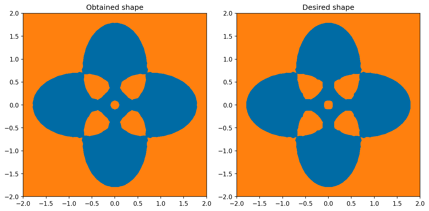
and the result looks like this As we can see, the BFGS method is able to reconstruct the desired clover shape after only about 100 iterations. We encourage readers to try the other (established) methods to compare the novel BFGS approach to established techniques and see that the new methods are significantly more efficient.

Note

The method plot_shape can be used to visualize the current shape based on the level-set function psi. Note that the cells inside \(\Omega\) are colored in yellow and the ones outside are colored blue.