cashocs as Solver for Shape Optimization Problems#

Problem Formulation#

Let us now investigate how cashocs can be used exclusively as a solver for shape optimization problems. The procedure is very similar to the one discussed in cashocs as Solver for Optimal Control Problems, but with some minor variations tailored to shape optimization.

As a model shape optimization problem we consider the same as in Shape Optimization with a Poisson Problem, i.e.,

\[\begin{split} \begin{align} &\min_\Omega J(u, \Omega) = \int_\Omega u \text{ d}x \\ &\text{subject to} \qquad \begin{alignedat}[t]{2} -\Delta u &= f \quad &&\text{ in } \Omega,\\ u &= 0 \quad &&\text{ on } \Gamma. \end{alignedat} \end{align} \end{split}\]

For the initial domain, we use the unit disc \(\Omega = \{ x \in \mathbb{R}^2 \,\mid\, \lvert\lvert x \rvert\rvert_2 < 1 \}\) and the right-hand side \(f\) is given by

\[ f(x) = 2.5 \left( x_1 + 0.4 - x_2^2 \right)^2 + x_1^2 + x_2^2 - 1. \]

Implementation#

The complete python code can be found in the file demo_shape_solver.py and the corresponding config can be found in config.ini.

Recapitulation of Shape Optimization with a Poisson Problem #

Analogously to cashocs as Solver for Optimal Control Problems, the code we use in case cashocs is treated as a solver only is identical to the one of Shape Optimization with a Poisson Problem up to the definition of the optimization problem. For the sake of completeness we recall the corresponding code in the following

from fenics import *

import cashocs

config = cashocs.load_config("./config.ini")

mesh, subdomains, boundaries, dx, ds, dS = cashocs.import_mesh("./mesh/mesh.xdmf")

V = FunctionSpace(mesh, "CG", 1)
u = Function(V)
p = Function(V)

x = SpatialCoordinate(mesh)
f = 2.5 * pow(x[0] + 0.4 - pow(x[1], 2), 2) + pow(x[0], 2) + pow(x[1], 2) - 1

e = inner(grad(u), grad(p)) * dx - f * p * dx
bcs = DirichletBC(V, Constant(0), boundaries, 1)

J = cashocs.IntegralFunctional(u * dx)

sop = cashocs.ShapeOptimizationProblem(e, bcs, J, u, p, boundaries, config=config)

Supplying Custom Adjoint Systems and Shape Derivatives#

Now, our goal is to use custom UFL forms for the adjoint system and shape derivative. Note, that the adjoint system for the considered optimization problem is given by

\[\begin{split} \begin{alignedat}{2} - \Delta p &= 1 \quad &&\text{ in } \Omega, \\ p &= 0 \quad &&\text{ on } \Gamma, \end{alignedat} \end{split}\]

and the corresponding shape derivative is given by

\[ dJ(\Omega)[\mathcal{V}] = \int_{\Omega} \text{div}\left( \mathcal{V} \right) u \text{ d}x + \int_{\Omega} \left( \left( \text{div}(\mathcal{V})I - 2 \varepsilon(\mathcal{V}) \right) \nabla u \right) \cdot \nabla p \text{ d}x + \int_{\Omega} \text{div}\left( f \mathcal{V} \right) p \text{ d}x, \]

where \(\varepsilon(\mathcal{V})\) is the symmetric part of the gradient of \(\mathcal{V}\), given by \(\varepsilon(\mathcal{V}) = \frac{1}{2} \left( D\mathcal{V} + D\mathcal{V}^\top \right)\). For details, we refer the reader to, e.g., Delfour and Zolesio - Shapes and Geometries.

To supply these weak forms to cashocs, we can use the following code. For the shape derivative, we write

def eps(u):
    return Constant(0.5) * (grad(u) + grad(u).T)


vector_field = sop.get_vector_field()
dJ = (
    div(vector_field) * u * dx
    - inner(
        (div(vector_field) * Identity(2) - 2 * eps(vector_field)) * grad(u),
        grad(p),
    )
    * dx
    + div(f * vector_field) * p * dx
)

Note, that we have to call the get_vector_field method which returns the UFL object corresponding to \(\mathcal{V}\) and which is to be used at its place.

Hint

Alternatively, one could define the variable vector_field as follows

space = VectorFunctionSpace(mesh, 'CG', 1)
vector_field = TestFunction(space)

which would yield identical results. However, the shorthand via the get_vector_field is more convenient, as one does not have to remember to define the correct function space first.

For the adjoint system, the procedure is exactly the same as in cashocs as Solver for Optimal Control Problems and we have the following code

adjoint_form = inner(grad(p), grad(TestFunction(V))) * dx - TestFunction(V) * dx
adjoint_bcs = bcs

Again, the format is analogous to the format of the state system, but now we have to specify a fenics.TestFunction object for the adjoint equation.

Finally, the weak forms are supplied to cashocs with the line

sop.supply_custom_forms(dJ, adjoint_form, adjoint_bcs)

and the optimization problem is solved with

sop.solve()

Note

One can also specify either the adjoint system or the shape derivative of the cost functional, using the methods supply_adjoint_forms or supply_derivatives. However, this is potentially dangerous, due to the following. The adjoint system is a linear system, and there is no fixed convention for the sign of the adjoint state. Hence, supplying, e.g., only the adjoint system, might not be compatible with the derivative of the cost functional which cashocs computes. In effect, the sign is specified by the choice of adding or subtracting the PDE constraint from the cost functional for the definition of a Lagrangian function, which is used to determine the adjoint system and derivative. cashocs internally uses the convention that the PDE constraint is added, so that, internally, it computes not the adjoint state \(p\) as defined by the equations given above, but \(-p\) instead. Hence, it is recommended to either specify all respective quantities with the supply_custom_forms method.

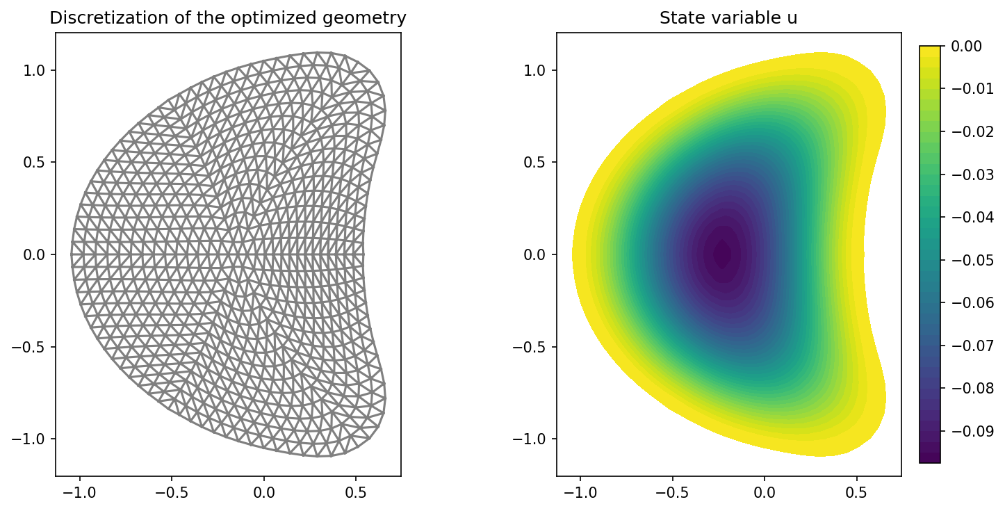
We visualize the results with the code

import matplotlib.pyplot as plt

plt.figure(figsize=(10, 5))

ax_mesh = plt.subplot(1, 2, 1)
fig_mesh = plot(mesh)
plt.title("Discretization of the optimized geometry")

ax_u = plt.subplot(1, 2, 2)
ax_u.set_xlim(ax_mesh.get_xlim())
ax_u.set_ylim(ax_mesh.get_ylim())
fig_u = plot(u)
plt.colorbar(fig_u, fraction=0.046, pad=0.04)
plt.title("State variable u")

plt.tight_layout()
# plt.savefig('./img_shape_solver.png', dpi=150, bbox_inches='tight')

The result is, of course, completely identical to the one of Shape Optimization with a Poisson Problem and looks as follows