Using Multiple Variables and PDEs#
Problem Formulation#
In this demo we show how cashocs can be used to treat multiple state equations as constraint. Additionally, this also highlights how the case of multiple controls can be treated. As model example, we consider the following problem
For the sake of simplicity, we restrict this investigation to homogeneous boundary conditions as well as to a very simple one way coupling. More complex problems (using e.g. Neumann control or more difficult couplings) are straightforward to implement.
In contrast to the previous examples, in the case where we have multiple state equations, which are either decoupled or only one-way coupled, the corresponding state equations are solved one after the other so that every input related to the state and adjoint variables has to be put into a ordered list, so that they can be treated properly, as is explained in the following.
Implementation#
The complete python code can be found in the file demo_multiple_variables.py
and the corresponding config can be found in config.ini.
Initialization#
The initial setup is identical to the previous cases (see, Distributed Control of a Poisson Problem), where we again use
from fenics import *

import cashocs

config = cashocs.load_config("config.ini")
mesh, subdomains, boundaries, dx, ds, dS = cashocs.regular_mesh(50)
V = FunctionSpace(mesh, "CG", 1)
which defines the geometry and the function space.
Definition of the problems#
We now first define the state equation corresponding to the state \(y\). This is done in analogy to Distributed Control of a Poisson Problem
y = Function(V)
p = Function(V)
u = Function(V)
e_y = inner(grad(y), grad(p)) * dx - u * p * dx
bcs_y = cashocs.create_dirichlet_bcs(V, Constant(0), boundaries, [1, 2, 3, 4])
Similarly to before, p is the adjoint state corresponding to y.
Next, we define the second state equation (which is for the state \(z\)) via
z = Function(V)
q = Function(V)
v = Function(V)
e_z = inner(grad(z), grad(q)) * dx - (y + v) * q * dx
bcs_z = cashocs.create_dirichlet_bcs(V, Constant(0), boundaries, [1, 2, 3, 4])
Here, q is the adjoint state corresponding to z.
In order to treat this one-way coupled with cashocs, we now have to specify what
the state, adjoint, and control variables are. This is done by putting the
corresponding fenics.Function objects into ordered lists
states = [y, z]
adjoints = [p, q]
controls = [u, v]
To define the corresponding state system, the state equations and Dirichlet boundary conditions also have to be put into an ordered list, i.e.,
e = [e_y, e_z]
bcs_list = [bcs_y, bcs_z]
Note
It is important, that the ordering of the state and adjoint variables, as well
as the state equations and boundary conditions is in the same way. This means,
that e[i] is the state equation for state[i], which is
supplemented with Dirichlet boundary conditions defined in bcs_list[i], and
has a corresponding adjoint state adjoints[i], for all i. In
analogy, the same holds true for the control variables, the scalar product of the
control space, and the control constraints, i.e., controls[j],
riesz_scalar_products[j], and control_constraints[j] all have to
belong to the same control variable.
Note that the control variables are completely independent of the state and adjoint ones, so that the relative ordering between these objects does not matter.
Defintion of the cost functional and optimization problem#
For the optimization problem we now define the cost functional via
y_d = Expression("sin(2*pi*x[0])*sin(2*pi*x[1])", degree=1)
z_d = Expression("sin(4*pi*x[0])*sin(4*pi*x[1])", degree=1)
alpha = 1e-6
beta = 1e-4
J = cashocs.IntegralFunctional(
    Constant(0.5) * (y - y_d) * (y - y_d) * dx
    + Constant(0.5) * (z - z_d) * (z - z_d) * dx
    + Constant(0.5 * alpha) * u * u * dx
    + Constant(0.5 * beta) * v * v * dx
)
This setup is sufficient to now define the optimal control problem and solve it, via
ocp = cashocs.OptimalControlProblem(
    e, bcs_list, J, states, controls, adjoints, config=config
)
ocp.solve()
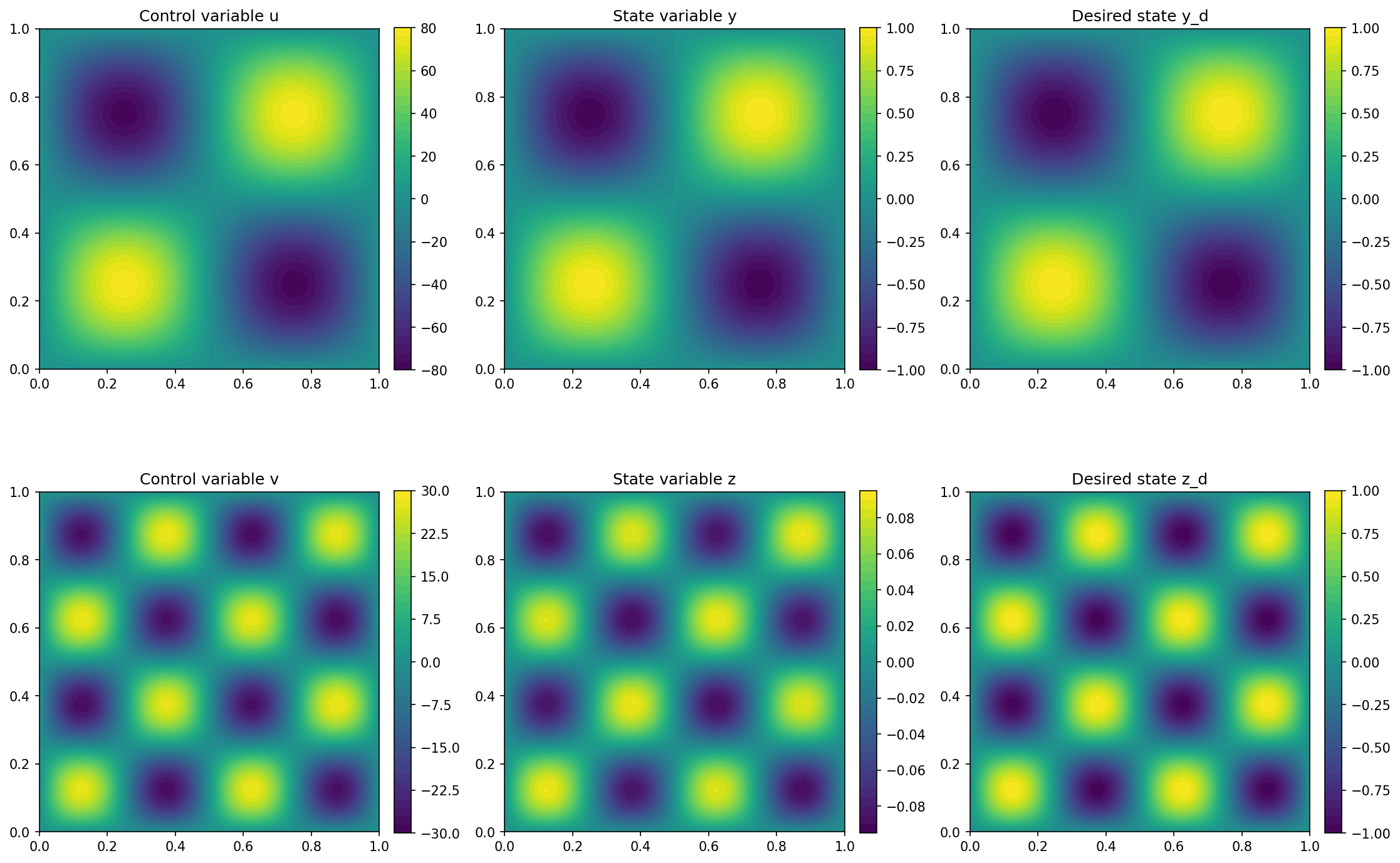
We visualize the results of the problem with the code
import matplotlib.pyplot as plt

plt.figure(figsize=(15, 10))

plt.subplot(2, 3, 1)
fig = plot(u)
plt.colorbar(fig, fraction=0.046, pad=0.04)
plt.title("Control variable u")

plt.subplot(2, 3, 2)
fig = plot(y)
plt.colorbar(fig, fraction=0.046, pad=0.04)
plt.title("State variable y")

plt.subplot(2, 3, 3)
fig = plot(y_d, mesh=mesh)
plt.colorbar(fig, fraction=0.046, pad=0.04)
plt.title("Desired state y_d")

plt.subplot(2, 3, 4)
fig = plot(v)
plt.colorbar(fig, fraction=0.046, pad=0.04)
plt.title("Control variable v")

plt.subplot(2, 3, 5)
fig = plot(z)
plt.colorbar(fig, fraction=0.046, pad=0.04)
plt.title("State variable z")

plt.subplot(2, 3, 6)
fig = plot(z_d, mesh=mesh)
plt.colorbar(fig, fraction=0.046, pad=0.04)
plt.title("Desired state z_d")

plt.tight_layout()
# plt.savefig('./img_multiple_variables.png', dpi=150, bbox_inches='tight')
and the output should look as follows
Note
Note, that the error between \(z\) and \(z_d\) is significantly larger
that the error between \(y\) and \(y_d\). This is due to the fact that
we use a different regularization parameter for the controls \(u\) and \(v\).
For the former, which only acts on \(y\), we have a regularization parameter
of alpha = 1e-6, and for the latter we have beta = 1e-4. Hence,
\(v\) is penalized higher for being large, so that also \(z\) is (significantly)
smaller than \(z_d\).
Hint
Note, that for the case that we consider control constraints (see Control Constraints) or different Hilbert spaces, e.g., for boundary control (see Neumann Boundary Control), the corresponding control constraints have also to be put into a joint list, i.e.,
cc_u = [u_a, u_b]
cc_v = [v_a, v_b]
cc = [cc_u, cc_v]
and the corresponding scalar products have to be treated analogously, i.e.,
scalar_product_u = TrialFunction(V)*TestFunction(V)*dx
scalar_product_v = TrialFunction(V)*TestFunction(V)*dx
scalar_products = [scalar_product_u, scalar_produt_v]
In summary, to treat multiple (control or state) variables, the
corresponding objects simply have to placed into ordered lists which
are then passed to the OptimalControlProblem
instead of the “single” objects as in the previous examples. Note, that each
individual object of these lists is allowed to be from a different function space,
and hence, this enables different discretizations of state and adjoint systems.