Coupled Problems - Picard Iteration#
Problem Formulation#
In this demo we show how cashocs can be used with a coupled PDE constraint. For this, we consider an iterative approach, whereas we investigated a monolithic approach in Coupled Problems - Monolithic Approach.
As model example, we consider the following problem
Again, the system is two-way coupled. To solve it, we now employ a Picard iteration. Therefore, the two PDEs are solved subsequently, where the variables are frozen in between: At the beginning the first PDE is solved for \(y\), with \(z\) being fixed. Afterwards, the second PDE is solved for \(z\) with \(y\) fixed. This is then repeated until convergence is reached.
Note
There is, however, no a-priori guarantee that the Picard iteration converges for a particular problem, unless a careful analysis is carried out by the user. Still, it is an important tool, which also often works well in practice.
Implementation#
The complete python code can be found in the file demo_picard_iteration.py
and the corresponding config can be found in config.ini.
Initialization#
The setup is as in Distributed Control of a Poisson Problem
from fenics import *

import cashocs

config = cashocs.load_config("config.ini")
mesh, subdomains, boundaries, dx, ds, dS = cashocs.regular_mesh(50)
V = FunctionSpace(mesh, "CG", 1)
However, compared to the previous examples, there is a major change in the config file. As we want to use the Picard iteration as solver for the state PDEs, we now specify
picard_iteration = True
see config.ini.
Definition of the state system#
The definition of the state system follows the same ideas as introduced in
Using Multiple Variables and PDEs: We define both state equations through their
components, and then gather them in lists, which are passed to the
OptimalControlProblem.
The state and adjoint variables are defined via
y = Function(V)
p = Function(V)
z = Function(V)
q = Function(V)
The control variables are defined as
u = Function(V)
v = Function(V)
Next, we define the state system, using the weak forms from Coupled Problems - Monolithic Approach
e_y = inner(grad(y), grad(p)) * dx + z * p * dx - u * p * dx
bcs_y = cashocs.create_dirichlet_bcs(V, Constant(0), boundaries, [1, 2, 3, 4])

e_z = inner(grad(z), grad(q)) * dx + y * q * dx - v * q * dx
bcs_z = cashocs.create_dirichlet_bcs(V, Constant(0), boundaries, [1, 2, 3, 4])
Finally, we use the same procedure as in Using Multiple Variables and PDEs, and put everything into (ordered) lists
states = [y, z]
adjoints = [p, q]
controls = [u, v]

e = [e_y, e_z]
bcs = [bcs_y, bcs_z]
Definition of the optimization problem#
The cost functional is defined as in Coupled Problems - Monolithic Approach, the only
difference is that y and z now are fenics.Function objects, whereas
they were generated with the ufl.split() command previously
y_d = Expression("sin(2*pi*x[0])*sin(2*pi*x[1])", degree=1)
z_d = Expression("sin(4*pi*x[0])*sin(4*pi*x[1])", degree=1)
alpha = 1e-6
beta = 1e-6
J = cashocs.IntegralFunctional(
    Constant(0.5) * (y - y_d) * (y - y_d) * dx
    + Constant(0.5) * (z - z_d) * (z - z_d) * dx
    + Constant(0.5 * alpha) * u * u * dx
    + Constant(0.5 * beta) * v * v * dx
)
Finally, we set up the optimization problem and solve it
optimization_problem = cashocs.OptimalControlProblem(
    e, bcs, J, states, controls, adjoints, config=config
)
optimization_problem.solve()
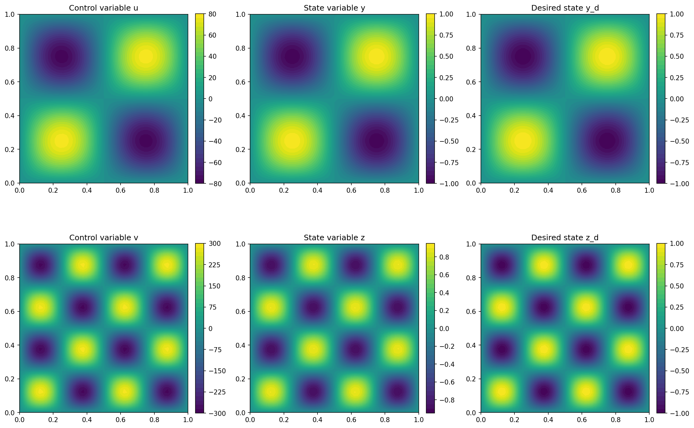
We visualize the results with the code
import matplotlib.pyplot as plt

plt.figure(figsize=(15, 10))

plt.subplot(2, 3, 1)
fig = plot(u)
plt.colorbar(fig, fraction=0.046, pad=0.04)
plt.title("Control variable u")

plt.subplot(2, 3, 2)
fig = plot(y)
plt.colorbar(fig, fraction=0.046, pad=0.04)
plt.title("State variable y")

plt.subplot(2, 3, 3)
fig = plot(y_d, mesh=mesh)
plt.colorbar(fig, fraction=0.046, pad=0.04)
plt.title("Desired state y_d")

plt.subplot(2, 3, 4)
fig = plot(v)
plt.colorbar(fig, fraction=0.046, pad=0.04)
plt.title("Control variable v")

plt.subplot(2, 3, 5)
fig = plot(z)
plt.colorbar(fig, fraction=0.046, pad=0.04)
plt.title("State variable z")

plt.subplot(2, 3, 6)
fig = plot(z_d, mesh=mesh)
plt.colorbar(fig, fraction=0.046, pad=0.04)
plt.title("Desired state z_d")

plt.tight_layout()
# plt.savefig('./img_picard_iteration.png', dpi=150, bbox_inches='tight')
and the result can be seen below
Note
Comparing the output (especially in the early iterations) between the monlithic and Picard apporach we observe that both methods yield essentially the same results (up to machine precision). This validates the Picard approach.
However, one should note that for this example, the Picard approach takes significantly longer to compute the optimizer. This is due to the fact that the individual PDEs have to be solved several times, whereas in the monolithic approach the state system is (slightly) larger, but has to be solved less often. However, the monolithic approach needs significantly more memory, so that the Picard iteration becomes feasible for very large problems. Further, the convergence properties of the Picard iteration are better, so that it may converge even when the monolithic approach fails.