Optimization of an Obstacle in Stokes Flow#
Problem Formulation#
For this tutorial, we investigate a problem similarly to the ones considered in, e.g., Blauth - Nonlinear Conjugate Gradient Methods for PDE Constrained Shape Optimization Based on Steklov-Poincaré-Type Metrics and Schulz and Siebenborn - Computational Comparison of Surface Metric for PDE Constrained Shape Optimization, which reads:
Here, we have an inflow boundary condition on the inlet \(\Gamma^\text{in}\), a no-slip boundary condition on the wall boundary \(\Gamma^\text{wall}\) as well as the obstacle boundary \(\Gamma^\text{obs}\), and a do-nothing condition on the outlet \(\Gamma^\text{out}\).
This problem is supplemented with the geometrical constraints
where \(\Omega_0\) denotes the initial geometry. This models that both the volume and the barycenter of the geometry should remain fixed during the optimization. To treat this problem with cashocs, we regularize the constraints in the sense of a quadratic penalty function. See the corresponding section in the documentation of the config files for shape optimization as well as Regularization for Shape Optimization Problems. In particular, the regularized problem reads
where we have no additional geometrical constraints. However, the parameters \(\mu_\text{vol}\) and \(\mu_\text{bary}\) have to be sufficiently large, so that the regularized constraints are satisfied approximately.
Note, that the domain \(\Omega\) denotes the domain of the obstacle, but that the cost functional involves an integral over the flow domain \(\Omega^\text{flow}\). Therefore, we switch our point of view and optimize the geometry of the flow instead (which of course includes the optimization of the “hole” generated by the obstacle). In particular, only the boundary of the obstacle \(\Gamma^\text{obs}\) is deformable, all remaining boundaries are fixed. Hence, it is equivalent to pose the geometrical constraints on \(\Omega\) and \(\Omega^\text{flow}\), so that we can work completely with the flow domain.
As (initial) domain, we consider the rectangle \((-2, 2) \times (-3, 3)\)
without a circle centered in the origin with radius \(0.5\). The correspondig
geometry is created with Gmsh, and can be found in the ./mesh/ directory.
Implementation#
The complete python code can be found in the file demo_shape_stokes.py,
and the corresponding config can be found in config.ini.
Initialization#
As for the previous tutorial problems, we start by importing FEniCS and cashocs and load the configuration file
from fenics import *

import cashocs

config = cashocs.load_config("./config.ini")
Afterwards we import the (initial) geometry with the import_mesh command
mesh, subdomains, boundaries, dx, ds, dS = cashocs.import_mesh("./mesh/mesh.xdmf")
Note
As defined in ./mesh/mesh.geo, we have the following boundaries
The inlet boundary \(\Gamma^\text{in}\), which has index
1The wall boundary \(\Gamma^\text{wall}\), which have index
2The outlet boundary \(\Gamma^\text{out}\), which has index
3The boundary of the obstacle \(\Gamma^\text{obs}\), which has index
4
To include the fact that only the obstacle boundary, with index 4, is
deformable, we have the following lines in the config file
[ShapeGradient]
shape_bdry_def = [4]
shape_bdry_fix = [1,2,3]
which ensures that only \(\Gamma^\text{obs}\) is deformable.
State system#
The definition of the state system is analogous to the one we considered in Distributed Control of a Stokes Problem. Here, we, too, use LBB stable Taylor-Hood elements, which are defined as
v_elem = VectorElement("CG", mesh.ufl_cell(), 2)
p_elem = FiniteElement("CG", mesh.ufl_cell(), 1)
V = FunctionSpace(mesh, MixedElement([v_elem, p_elem]))
For the weak form of the PDE, we have the same code as in Distributed Control of a Stokes Problem
up = Function(V)
u, p = split(up)
vq = Function(V)
v, q = split(vq)

e = inner(grad(u), grad(v)) * dx - p * div(v) * dx - q * div(u) * dx
The Dirichlet boundary conditions are slightly different, though. For the inlet velocity \(u^\text{in}\) we use a parabolic profile
u_in = Expression(("-1.0/4.0*(x[1] - 2.0)*(x[1] + 2.0)", "0.0"), degree=2)
bc_in = DirichletBC(V.sub(0), u_in, boundaries, 1)
The wall and obstacle boundaries get a no-slip boundary condition, each, with the line
bc_no_slip = cashocs.create_dirichlet_bcs(
    V.sub(0), Constant((0, 0)), boundaries, [2, 4]
)
Finally, all Dirichlet boundary conditions are gathered into the list bcs
bcs = [bc_in] + bc_no_slip
Note
The outflow boundary condition is of Neumann type and already included in the weak form of the problem.
Cost functional and optimization problem#
The cost functional is easily defined with the line
J = cashocs.IntegralFunctional(inner(grad(u), grad(u)) * dx)
Note
The additional regularization terms are defined similarly to Regularization for Shape Optimization Problems. In the config file, we have the following (relevant) lines:
[Regularization]
factor_volume = 1e4
use_initial_volume = True
factor_barycenter = 1e5
use_initial_barycenter = True
This ensures that we use \(\mu_\text{vol} = 1e4\) and \(\mu_\text{bary} = 1e5\),
which are comparatively large parameters, so that the geometrical constraints are
satisfied with high accuracy.
Moreover, the boolean flags use_initial_volume and
use_initial_barycenter, which are both set to True, ensure that we actually
use the volume and barycenter of the initial geometry.
Finally, we solve the shape optimization problem as previously with the commands
sop = cashocs.ShapeOptimizationProblem(e, bcs, J, up, vq, boundaries, config=config)
sop.solve()
Note
For the definition of the shape gradient, we use the same parameters for the linear elasticity equations as in Blauth - Nonlinear Conjugate Gradient Methods for PDE Constrained Shape Optimization Based on Steklov-Poincaré-Type Metrics and Schulz and Siebenborn - Computational Comparison of Surface Metric for PDE Constrained Shape Optimization. These are defined in the config file in the ShapeGradient section
[ShapeGradient]
lambda_lame = 0.0
damping_factor = 0.0
mu_fix = 1
mu_def = 5e2
so that we use a rather high stiffness for the elements at the deformable boundary, which is also discretized finely, and a rather low stiffness for the fixed boundaries.
Note
This demo might take a little longer than the others, depending on the machine it is run on. This is normal, and caused by the finer discretization of the geometry compared to the previous problems.
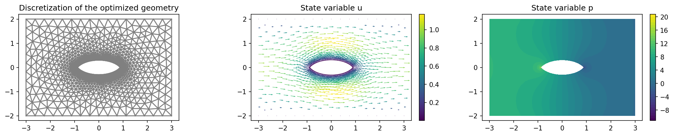
We visualize the optimized geometry with the lines
import matplotlib.pyplot as plt

plt.figure(figsize=(15, 3))

ax_mesh = plt.subplot(1, 3, 1)
fig_mesh = plot(mesh)
plt.title("Discretization of the optimized geometry")

ax_u = plt.subplot(1, 3, 2)
ax_u.set_xlim(ax_mesh.get_xlim())
ax_u.set_ylim(ax_mesh.get_ylim())
fig_u = plot(u)
plt.colorbar(fig_u, fraction=0.046, pad=0.04)
plt.title("State variable u")


ax_p = plt.subplot(1, 3, 3)
ax_p.set_xlim(ax_mesh.get_xlim())
ax_p.set_ylim(ax_mesh.get_ylim())
fig_p = plot(p)
plt.colorbar(fig_p, fraction=0.046, pad=0.04)
plt.title("State variable p")

plt.tight_layout()
# plt.savefig('./img_shape_stokes.png', dpi=150, bbox_inches='tight')
and the result is shown below