Space Mapping Shape Optimization - Uniform Flow Distribution#
Problem Formulation#
Let us consider another example of the space mapping technique, this time with an application to fluid dynamics. For an introduction to the space mapping technique, we refer the reader, e.g., to Bakr, Bandler, Madsen, Sondergaard - An Introduction to the Space Mapping Technique and Echeverria and Hemker - Space mapping and defect correction. For a detailed description of the methods in the context of shape optimization, we refer to Blauth - Space Mapping for PDE Constrained Shape Optimization.
The example is taken from Blauth - Space Mapping for PDE Constrained Shape Optimization and we refer the reader to this publication for a detailed discussion of the problem setup.
Assume that we have a pipe system consisting of one inlet \(\Gamma_\mathrm{in}\) and three outlets \(\Gamma_\mathrm{out}^i\) for \(i=1,2,3\). The geometry of the pipe is denoted by \(\Omega\) and the wall of the pipe is denoted by \(\Gamma_\mathrm{wall}\). A sketch of this problem is shown below
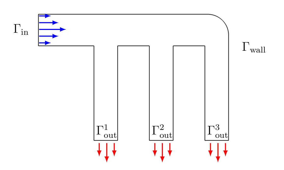
We consider the optimization of the pipe system so that the flow of some fluid becomes uniform over all three outlets. Therefore, let \(u\) denote the fluid’s velocity. The outlet flow rate \(q_\mathrm{out}^i(u)\) over pipe \(i\) is defined as
Therefore, we can define our optimization problem as follows
Here, we use the incompressible Navier-Stokes equations as PDE constraint. Note that the above model plays the role of the fine model, which is the problem we are interested in solving.
However, as solving the nonlinear Navier-Stokes equations can be difficult and time-consuming, we use a coarse model consisting of the linear Stokes system, so that the coarse model optimization problem is given by
Note
Again, we need a misalignment function to match the fine and coarse model responses, see Space Mapping Shape Optimization - Semilinear Transmission Problem. For this problem, we use the misalignment function
so that the parameter extraction problem which has to be solved in each iteration of the space mapping method reads
Implementation#
The complete python code can be found in the file
demo_space_mapping_uniform_flow_distribution.py
and the corresponding config can be found in config.ini.
The coarse model#
As in Space Mapping Shape Optimization - Semilinear Transmission Problem, we start with the implementation of the coarse model. We start by importing the required packages
import ctypes
import os
import subprocess

from fenics import *

import cashocs
and we will detail why we require the packages when they are used. Next, we define the space mapping module, set up the log level, and define the current working directory
space_mapping = cashocs.space_mapping.shape_optimization
cashocs.set_log_level(cashocs.log.ERROR)
dir = os.path.dirname(os.path.realpath(__file__))
We then define the Reynolds number \(\mathrm{Re} = 100\) and load the configuration file for the problem
Re = 100.0
cfg = cashocs.load_config("./config.ini")
In the next steps, we define the coarse model, in analogy to all of the previous demos (see, e.g., Optimization of an Obstacle in Stokes Flow
mesh, subdomains, boundaries, dx, ds, dS = cashocs.import_mesh("./mesh/mesh.xdmf")
n = FacetNormal(mesh)

u_in = Expression(("6.0*(0.0 - x[1])*(x[1] + 1.0)", "0.0"), degree=2)
q_in = -assemble(dot(u_in, n) * ds(1))
output_list = []

v_elem = VectorElement("CG", mesh.ufl_cell(), 2)
p_elem = FiniteElement("CG", mesh.ufl_cell(), 1)
V = FunctionSpace(mesh, v_elem * p_elem)

up = Function(V)
u, p = split(up)
vq = Function(V)
v, q = split(vq)

F = inner(grad(u), grad(v)) * dx - p * div(v) * dx - q * div(u) * dx
bc_in = DirichletBC(V.sub(0), u_in, boundaries, 1)
bcs_wall = cashocs.create_dirichlet_bcs(
    V.sub(0), Constant((0.0, 0.0)), boundaries, [2, 3, 4]
)
bc_out = DirichletBC(V.sub(0).sub(0), Constant(0.0), boundaries, 5)
bc_pressure = DirichletBC(V.sub(1), Constant(0.0), boundaries, 5)
bcs = [bc_in] + bcs_wall + [bc_out] + [bc_pressure]

J = [cashocs.ScalarTrackingFunctional(dot(u, n) * ds(i), q_in / 3) for i in range(5, 8)]

coarse_model = space_mapping.CoarseModel(F, bcs, J, up, vq, boundaries, config=cfg)
Note
The difference between the standard cashocs syntax and the syntax for space mapping is
that we now use CoarseModel instead of the usual
ShapeOptimizationProblem.
Note
The boundary conditions consist of a prescribed flow at the inlet. In order to be compatible with the incompressibility condition, we need to have that the outlet flow rates sum up to the inlet flow rate, so that mass is neither created nor destroyed. Of course, one could use a target output flow rate which does not satisfy this condition, but this would be unphysical. Therefore, the boundary condition on the inlet is defined as
u_in = Expression(("6.0*(0.0 - x[1])*(x[1] + 1.0)", "0.0"), degree=2)
bc_in = DirichletBC(V.sub(0), u_in, boundaries, 1)
q_in = -assemble(dot(u_in, n) * ds(1))
and the cost functional is given by
J = [cashocs.ScalarTrackingFunctional(dot(u, n) * ds(i), q_in / 3) for i in range(5, 8)]
so that the target outlet flow rate is given by q_in / 3, which means that
we have a uniform flow distribution. For more details regrading the usage of
ScalarTrackingFunctional, we refer to
Tracking of Scalar Functionals for Optimal Control Problems.
The fine model#
As next step, we define the fine model optimization problem as follows
class FineModel(space_mapping.FineModel):
    def __init__(self, mesh, Re, q_in, output_list):
        super().__init__(mesh)

        self.tracking_goals = [ctypes.c_double(0.0) for _ in range(5, 8)]

        self.iter = 0
        self.Re = Re
        self.q_in = q_in
        self.output_list = output_list

    def solve_and_evaluate(self):
        self.iter += 1

        # write out the mesh
        cashocs.io.write_out_mesh(
            self.mesh, "./mesh/mesh.msh", f"./mesh/fine/mesh_{self.iter}.msh"
        )
        cashocs.io.write_out_mesh(self.mesh, "./mesh/mesh.msh", f"./mesh/fine/mesh.msh")

        subprocess.run(
            ["gmsh", "./mesh/fine.geo", "-2", "-o", "./mesh/fine/fine.msh"],
            check=True,
            stdout=subprocess.DEVNULL,
            stderr=subprocess.DEVNULL,
        )
        cashocs.convert("./mesh/fine/fine.msh", "./mesh/fine/fine.xdmf")

        mesh, subdomains, boundaries, dx, ds, dS = cashocs.import_mesh(
            "./mesh/fine/fine.xdmf"
        )
        n = FacetNormal(mesh)
        v_elem = VectorElement("CG", mesh.ufl_cell(), 2)
        p_elem = FiniteElement("CG", mesh.ufl_cell(), 1)
        V = FunctionSpace(mesh, v_elem * p_elem)

        up = Function(V)
        u, p = split(up)
        v, q = TestFunctions(V)

        F = (
            inner(grad(u), grad(v)) * dx
            + Constant(self.Re) * inner(grad(u) * u, v) * dx
            - p * div(v) * dx
            - q * div(u) * dx
        )

        u_in = Expression(("6.0*(0.0 - x[1])*(x[1] + 1.0)", "0.0"), degree=2)
        bc_in = DirichletBC(V.sub(0), u_in, boundaries, 1)
        bcs_wall = cashocs.create_dirichlet_bcs(
            V.sub(0), Constant((0.0, 0.0)), boundaries, [2, 3, 4]
        )
        bc_out = DirichletBC(V.sub(0).sub(0), Constant(0.0), boundaries, 5)
        bc_pressure = DirichletBC(V.sub(1), Constant(0.0), boundaries, 5)
        bcs = [bc_in] + bcs_wall + [bc_out] + [bc_pressure]

        cashocs.snes_solve(F, up, bcs)
        self.u, p = up.split(True)

        file = File(f"./pvd/u_{self.iter}.pvd")
        file.write(self.u)

        J_list = [
            cashocs.ScalarTrackingFunctional(dot(self.u, n) * ds(i), self.q_in / 3)
            for i in range(5, 8)
        ]
        self.cost_functional_value = cashocs._utils.summation(
            [J.evaluate() for J in J_list]
        )

        self.flow_values = [assemble(dot(self.u, n) * ds(i)) for i in range(5, 8)]
        self.output_list.append(self.flow_values)

        for idx in range(len(self.tracking_goals)):
            self.tracking_goals[idx].value = self.flow_values[idx]


fine_model = FineModel(mesh, Re, q_in, output_list)
Again, the fine model problem is defined by subclassing FineModel and overwriting its
solve_and_evaluate
method.
Description of the FineModel
Let us investigate the fine model in more details in the following. The fine models
initialization starts with a call to its parent’s __init__() method, where
the mesh is passed
super().__init__(mesh)
Next, a list of tracking goals is defined using the ctypes module
self.tracking_goals = [ctypes.c_double(0.0) for _ in range(5, 8)]
Note
The ctypes module allows us to make floats in python mutable, i.e., to
behave like pointers. This is needed for the parameter extraction step, where we want
to find a coarse model “optimum” which achieves the same flow rates as the current
iterate of the fine model. In particular, the list self.tracking_goals will
be used later as input for the parameter extraction.
Afterwards, we have standard initializations of an iteration counter, the Reynolds number, the inlet flow rate, and an output list, which will be used to save the progress of the space mapping method
self.iter = 0
self.Re = Re
self.q_in = q_in
self.output_list = output_list
Let us now take a look at the core of the fine model, its solve_and_evaluate
method. It starts by incrementing the iteration counter
self.iter += 1
Next, the current mesh is exported to two Gmsh .msh files. The first is used for a possible post-processing (so that the evolution of the geometries is saved) whereas the second is used to define the fine model mesh
cashocs.io.write_out_mesh(
    self.mesh, "./mesh/mesh.msh", f"./mesh/fine/mesh_{self.iter}.msh"
)
cashocs.io.write_out_mesh(self.mesh, "./mesh/mesh.msh", f"./mesh/fine/mesh.msh")
Note that we do not use the same discretization for the fine and coarse model in this
problem, but we remesh the geometry of the fine model using a higher resolution. To do
so, the following Gmsh command is used, which is invoked via the subprocess
module
subprocess.run(
    ["gmsh", "./mesh/fine.geo", "-2", "-o", "./mesh/fine/fine.msh"],
    check=True,
    stdout=subprocess.DEVNULL,
    stderr=subprocess.DEVNULL,
)
Finally, the mesh generated with the above command is converted to XDMF with
cashocs.convert()
cashocs.convert("./mesh/fine/fine.msh", "./mesh/fine/fine.xdmf")
Now that we have the geometry of the problem, it is loaded into python and we define the Taylor-Hood Function Space for the Navier-Stokes system
mesh, subdomains, boundaries, dx, ds, dS = cashocs.import_mesh(
    "./mesh/fine/fine.xdmf"
)
n = FacetNormal(mesh)
v_elem = VectorElement("CG", mesh.ufl_cell(), 2)
p_elem = FiniteElement("CG", mesh.ufl_cell(), 1)
V = FunctionSpace(mesh, v_elem * p_elem)

up = Function(V)
u, p = split(up)
v, q = TestFunctions(V)
Next, we define the weak form of the problem and its boundary conditions
F = (
    inner(grad(u), grad(v)) * dx
    + Constant(self.Re) * inner(grad(u) * u, v) * dx
    - p * div(v) * dx
    - q * div(u) * dx
)

u_in = Expression(("6.0*(0.0 - x[1])*(x[1] + 1.0)", "0.0"), degree=2)
bc_in = DirichletBC(V.sub(0), u_in, boundaries, 1)
bcs_wall = cashocs.create_dirichlet_bcs(
    V.sub(0), Constant((0.0, 0.0)), boundaries, [2, 3, 4]
)
bc_out = DirichletBC(V.sub(0).sub(0), Constant(0.0), boundaries, 5)
bc_pressure = DirichletBC(V.sub(1), Constant(0.0), boundaries, 5)
bcs = [bc_in
The problem is then solved with <cashocs.snes_solve>()
cashocs.snes_solve(F, up, bcs)
Finally, after having solved the problem, we first save the solution for later visualization by
self.u, p = up.split(True)

file = File(f"./pvd/u_{self.iter}.pvd")
file.write(self.u)
Next, we evaluate the cost functional with the lines
J_list = [
    cashocs.ScalarTrackingFunctional(dot(self.u, n) * ds(i), self.q_in / 3)
    for i in range(5, 8)
]
self.cost_functional_value = cashocs._utils.summation(
    [J.evaluate() for J in J_list]
)
Finally, we save the values of the outlet flow rate first to our list
self.output_list and second to the list self.tracking_goals, so
that the parameter extraction can see the updated flow rates
self.flow_values = [assemble(dot(self.u, n) * ds(i)) for i in range(5, 8)]
self.output_list.append(self.flow_values)

for idx in range(len(self.tracking_goals)):
    self.tracking_goals[idx].value = self.flow_values[idx]
Note that we have to overwrite self.tracking_goals[idx].value as
self.tracking_goals[idx] is a ctypes.double object.
Attention
As already mentioned in Space Mapping Shape Optimization - Semilinear Transmission Problem, users have
to update the attribute cost_functional_value of the fine model in order
for the space mapping method to be able to use the value.
Parameter Extraction#
Now, we are finally ready to define the parameter extraction. This is done via
up_param = Function(V)
u_param, p_param = split(up_param)
J_param = [
    cashocs.ScalarTrackingFunctional(
        dot(u_param, n) * ds(i), fine_model.tracking_goals[idx]
    )
    for idx, i in enumerate(range(5, 8))
]
parameter_extraction = space_mapping.ParameterExtraction(
    coarse_model, J_param, up_param, config=cfg
)
Note
The parameter extraction uses the previously defined list
fine_model.tracking_goals of type ctypes.double for the
definition of its cost functional.
Space Mapping Problem and Solution#
In the end, we can now define the space mapping problem and solve it with the lines
problem = space_mapping.SpaceMappingProblem(
    fine_model,
    coarse_model,
    parameter_extraction,
    method="broyden",
    max_iter=25,
    tol=1e-4,
    use_backtracking_line_search=False,
    broyden_type="good",
    memory_size=5,
    save_history=True,
)
problem.solve()
We visualize the results with the code
import matplotlib.pyplot as plt

plt.figure(figsize=(20, 20))

ax_coarse = plt.subplot(2, 2, 1)
fig_coarse = plot(mesh)
plt.title("Coarse Model Optimal Mesh")

ax_fine = plt.subplot(2, 2, 2)
fig_fine = plot(fine_model.u.function_space().mesh())
plt.title("Fine Model Optimal Mesh")

ax_coarse2 = plt.subplot(2, 2, 3)
fig_coarse2 = plot(u)
plt.title("Velocity (coarse model)")

ax_fine2 = plt.subplot(2, 2, 4)
fig_fine2 = plot(fine_model.u)
plt.title("Velocity (fine model)")

plt.tight_layout()
# plt.savefig(
#     "./img_space_mapping_uniform_flow_distribution.png", dpi=150, bbox_inches="tight"
# )
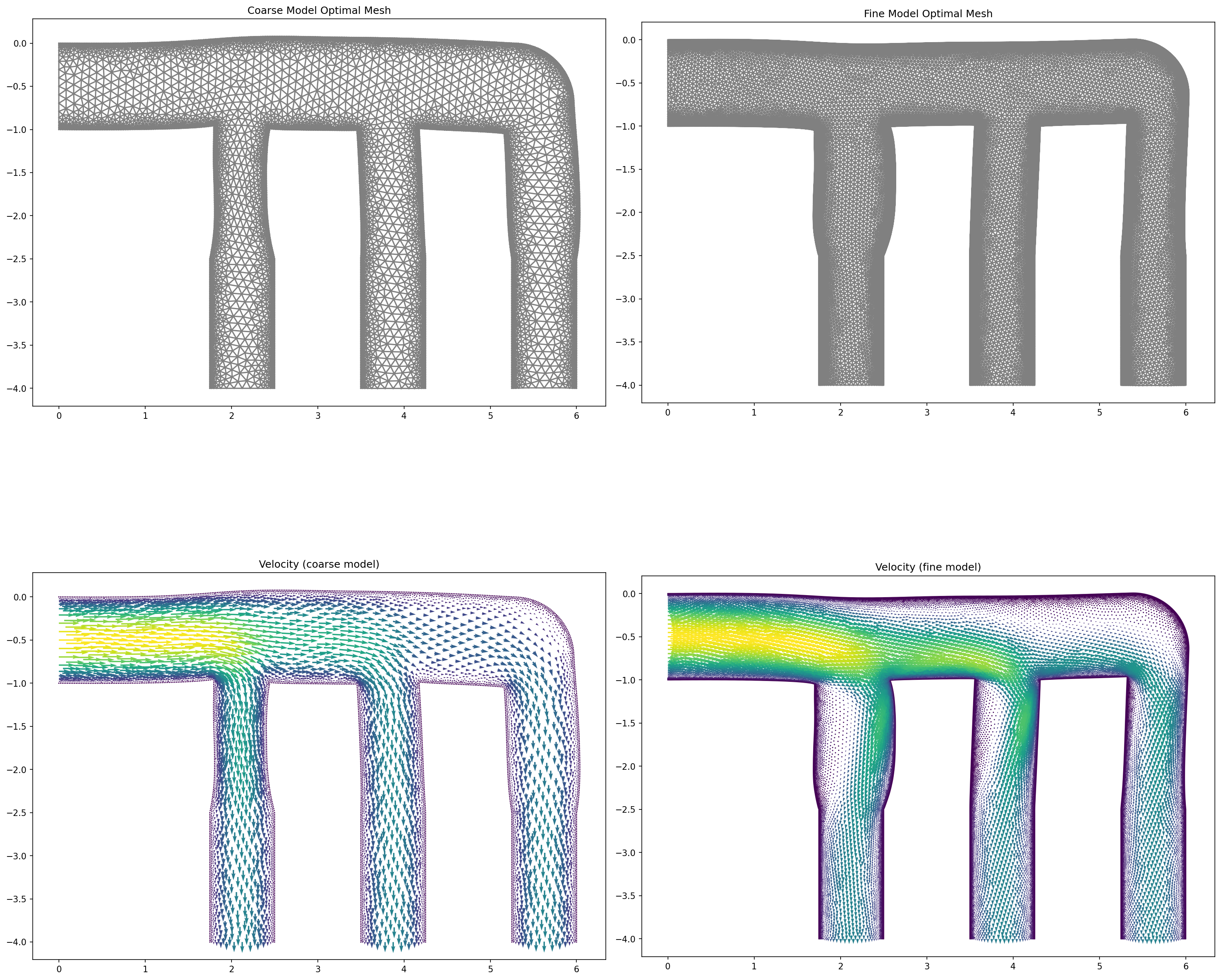
and the output is shown below
Note
On the left side of the above image the results for the coarse model are shown, whereas the results for the fine model are shown on the left side. On the top of the figure we see the geometries used for the models, and on the bottom the velocity is shown.
We observe that the coarse model uses a much coarser discretization in comparison with the fine model. Moreover, we can also nicely see that the coarse model optimal geometry works fine for optimizing the Stokes system, but that the behavior of the fine model is vastly different due to the inertial effects of the Navier-Stokes system. However, the space mapping technique still allows us to solve the fine model problem with the help of the approximate coarse model, where we only require simulations of the fine model.
For a more thorough discussion of the results, we refer the reader to Blauth - Space Mapping for PDE Constrained Shape Optimization.