Mesh Quality Constraints for Shape Optimization#
Problem Formulation#
In this demo, we demonstrate cashocs capability of enforcing a certain mesh quality, which is given by the user. As model problem, we consider the one already considered in Shape Optimization with a Poisson Problem, which we briefly recall here
For the initial domain, we use the unit disc \(\Omega = \{ x \in \mathbb{R}^2 \,\mid\, \lvert\lvert x \rvert\rvert_2 < 1 \}\) and the right-hand side \(f\) is given by
Mesh Quality Constraints#
Our software cashocs has the option to enforce a certain mesh quality during the shape optimization. This is done by adding additional equality and inequality constraints, which act on the discretized geometry, i.e., the finite element mesh. These constraints are of the form
where \(\alpha\) is some angle (in the case of a 2D triangular mesh) or dihedral angle (for a 3D tetrahedral mesh) and \(c\) is a lower bound for this angle. Note that this constraint is posed for all angles \(\alpha\) in the mesh (which is denoted by \(\Omega_h\)).
Note
Note that many mesh quality criteria are either explicitly or implictly dependent on
the (dihedral) angle of the mesh elements. For examples, we refer the reader to
cashocs.geometry.quality. As a concrete example, consider the so-called
skewness of the mesh, which is given by
It is easy to see, that this is maximal (i.e. has the value 1) for \(\alpha = \alpha^*\) and that the mesh quality deteriorates (i.e. it goes to 0) for either \(\alpha \to 0\) or \(\alpha \to \pi\).
With the help of the above constraint, the skewness of some triangular mesh is bounded by
due to the fact that the above constraint implies that \(\alpha \leq \pi - 2c\) for a triangular mesh (the sum of all triangular angles is \(\pi\)). A similar observation also holds true for a tetrahedral mesh (there, the sum of the dihedral angles is bounded between \(2\pi\) and \(3\pi\)).
For this reason, the above constraints enforce the quality in the mesh in the sense that no element can become degenerate during the optimization if the constraints are satisfied.
Note
Note that for some meshes it might not be sensible to define the lower threshold for the (dihedral) angle globally, i.e., use a single value of \(c\) for all cells, for example when using stretched elements for resolving boundary layers. Therefore, cashocs can either use a globally defined threshold \(c > 0\) or a value of \(c\) which is different for each cell in the mesh and depends on the angles in the initial mesh. In the latter case, the user can specify a factor \(\varphi \in (0,1)\) and \(c\) in element \(k\) is chosen as \(c_k = \phi \min_i \alpha_i\), i.e., it is chosen as \(\varphi\) times the minimum angle of the element. This choice still preserves the mesh quality as it ensures that the elements can not deteriorate.
Of course, the constraints can only be satisfied up to a numerical tolerance, so that this tolerance also needs to be specified by the user. It is suggested that users try the default tolerance of 1e-2 first. For some problems, a larger tolerance, e.g., 1e-1 might yield faster results, but sometimes it might be necessary to use a tighter tolerance.
Implementation#
The complete python code can be found in the file
demo_mesh_quality_constraints.py,
and the corresponding config can be found in config.ini.
Solving the Problem without Mesh Quality Constraints#
Let us first consider solving the above problem without any mesh quality to see what happens. To do so, we follow Shape Optimization with a Poisson Problem, with some minor modifications.
from fenics import *

import cashocs

print("### Optimization without Mesh Quality Constraints ###")
cashocs.set_log_level(cashocs.LogLevel.INFO)
config = cashocs.load_config("./config.ini")

mesh, subdomains, boundaries, dx, ds, dS = cashocs.import_mesh("./mesh/mesh.xdmf")

initial_mesh_quality = cashocs.compute_mesh_quality(mesh)

V = FunctionSpace(mesh, "CG", 1)
u = Function(V)
p = Function(V)

x = SpatialCoordinate(mesh)
f = 2.5 * pow(x[0] + 0.4 - pow(x[1], 2), 2) + pow(x[0], 2) + pow(x[1], 2) - 1

e = inner(grad(u), grad(p)) * dx - f * p * dx
bcs = DirichletBC(V, Constant(0), boundaries, 1)

J = cashocs.IntegralFunctional(u * dx)

sop = cashocs.ShapeOptimizationProblem(e, bcs, J, u, p, boundaries, config=config)
sop.solve()

optimized_mesh_quality = cashocs.compute_mesh_quality(mesh)
print(f"Quality of the initial mesh: {initial_mesh_quality:.3e}")
print(f"Quality of the optimized mesh: {optimized_mesh_quality:.3e}")
This code is the same as before, the only difference is that the mesh quality for the initial and optimized meshes is computed and printed to the console. The output is given by
Quality of the initial mesh: 6.391e-01
Quality of the optimized mesh: 4.831e-01
Hence, we observe that the mesh quality goes down quite a bit. Of course, the quality of the optimized mesh is still acceptable, nevertheless we use this as an example to show how cashocs can preserve the mesh quality.
Solving the Problem with Mesh Quality Constraints#
For using the mesh quality constraints, the user only has to change the configuration file. To make this more obvious, we load the config file into the python script and modify the corresponding values directly there. Hence, our setup is very similar to before, i.e.,
from fenics import *

import cashocs

print("### Optimization with Mesh Quality Constraints ###")
cashocs.set_log_level(cashocs.LogLevel.INFO)
config = cashocs.load_config("./config.ini")

mesh, subdomains, boundaries, dx, ds, dS = cashocs.import_mesh("./mesh/mesh.xdmf")

initial_mesh_quality = cashocs.compute_mesh_quality(mesh)

V = FunctionSpace(mesh, "CG", 1)
u = Function(V)
p = Function(V)

x = SpatialCoordinate(mesh)
f = 2.5 * pow(x[0] + 0.4 - pow(x[1], 2), 2) + pow(x[0], 2) + pow(x[1], 2) - 1

e = inner(grad(u), grad(p)) * dx - f * p * dx
bcs = DirichletBC(V, Constant(0), boundaries, 1)

J = cashocs.IntegralFunctional(u * dx)
To specify the mesh quality constraints, we now modify the corresponding parameters in the configuration with the following line. We only have specify the minimum angle of the elements (in degrees) which is done with
config.set("MeshQualityConstraints", "min_angle", "35.0")
A minimum angle of 35°, as specified above, leads to a minimum skewness of the mesh of
0.5833 and since we consider a tolerance of 1e-2, this means that we can
expect a minimum skewness of 0.5733 for the mesh.
Warning
Mesh quality constraints are implemented for all available methods for shape optimization, i.e., the gradient descent, nonlinear CG, and BFGS methods. However, the theory only works for the gradient descent method at the moment. Numerical examples suggest, that the method also works well with the NCG and BFGS methods, but there is no guarantee that this works, so use this with some care only.
Note
As we are solving the problem numerically, the constraints can only be satisfied up to a certain numerical tolerance. This can be specified with the line
config.set("MeshQualityConstraints", "tol", "1e-2")
A value of 1e-2 is the default and should work reasonably well for most problems. If
the constraint handling takes too much time, a higher tolerance of 1e-1 might be
useful for some problems. On the other hand, for problems requiring more strict
handling of the constraints, a lower tolerance, such as 1e-3, could be beneficial.
Note
If one has a non-uniform mesh, e.g., for resolving boundary layers, then the user can, as explained above, define a factor \(\varphi \in (0,1)\) which the angles of some element can become smaller. This can be done with the configuration parameter
cfg.set("MeshQualityConstraints", "feasible_angle_reduction_factor", "0.5")
This means that all (dihedral) angles of the mesh can become half (or a factor of \(\varphi\) in general) of the minimum angle of the respective element.
If both a feasible_angle_reduction_factor and min_angle are specified,
then the minimum of both (on a per-element basis) is used to ensure that the initial
mesh is feasible w.r.t. the constraints.
Finally, we can solve this problem with the lines
sop = cashocs.ShapeOptimizationProblem(e, bcs, J, u, p, boundaries, config=config)
sop.solve()
To compare the solution with the mesh quality constraints, we also compute the mesh quality of the optimized mesh with the lines
optimized_mesh_quality = cashocs.compute_mesh_quality(mesh)
print(f"Quality of the initial mesh: {initial_mesh_quality:.3e}")
print(f"Quality of the optimized mesh: {optimized_mesh_quality:.3e}")
and we get the following output
Quality of the initial mesh: 6.391e-01
Quality of the optimized mesh: 5.751e-01
i.e. the mesh quality constraints have been successful in enforcing a higher mesh
quality. In particular, we observe that the minimum allowed skewness of 0.5733 is,
in fact, (numerically) achieved for the optimized mesh.
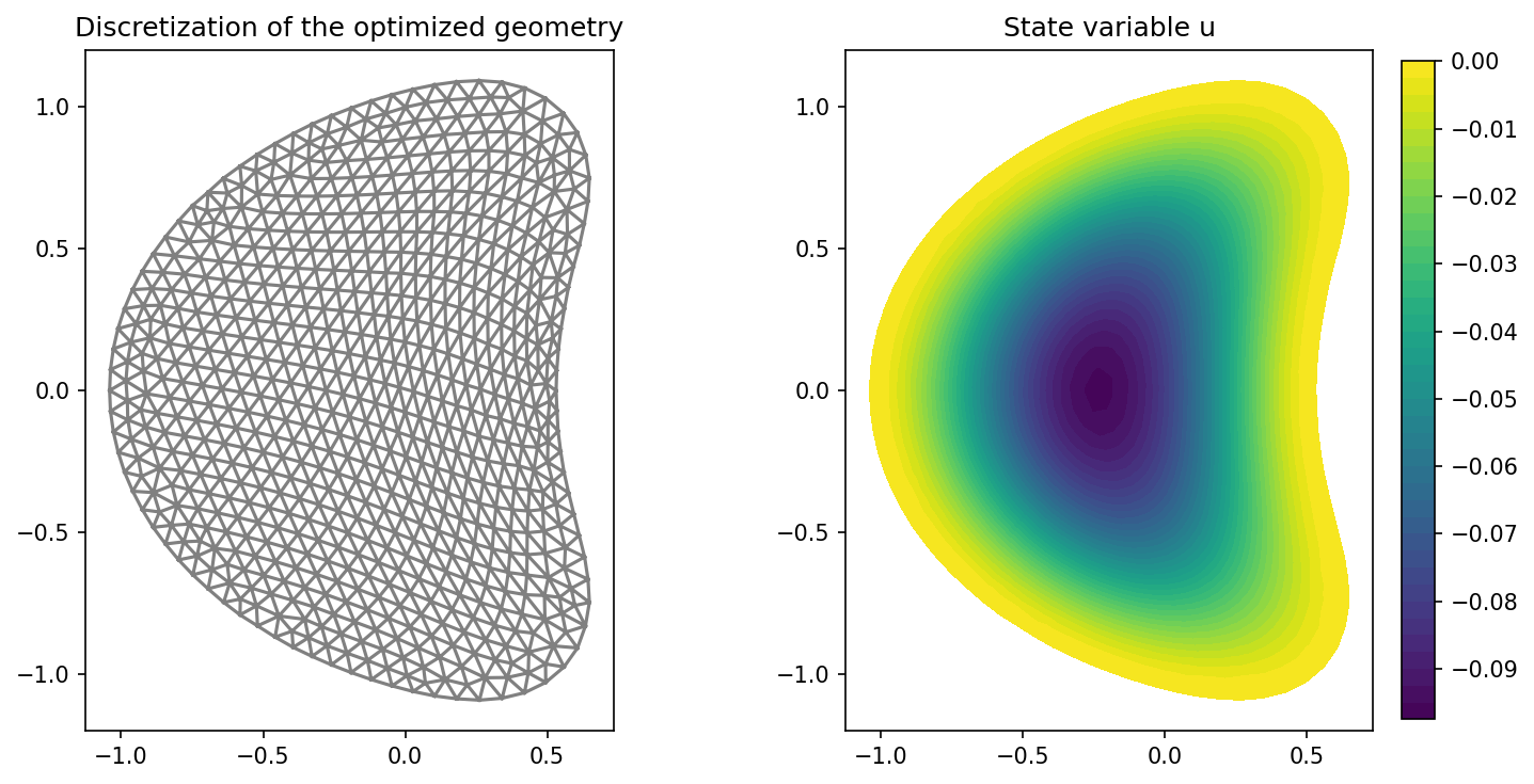
Finally, we visualize the result with the following code
import matplotlib.pyplot as plt

plt.figure(figsize=(10, 5))

ax_mesh = plt.subplot(1, 2, 1)
fig_mesh = plot(mesh)
plt.title("Discretization of the optimized geometry")

ax_u = plt.subplot(1, 2, 2)
ax_u.set_xlim(ax_mesh.get_xlim())
ax_u.set_ylim(ax_mesh.get_ylim())
fig_u = plot(u)
plt.colorbar(fig_u, fraction=0.046, pad=0.04)
plt.title("State variable u")

plt.tight_layout()
# plt.savefig("./img_mesh_quality_constraints.png", dpi=150, bbox_inches="tight")
and the result should look like this