Computing the Shape Stiffness via Distance to the Boundaries

Problem Formulation

We are solving the same problem as in Optimization of an Obstacle in Stokes Flow, but now use a different approach for computing the stiffness of the shape gradient. Recall, that the corresponding (regularized) shape optimization problem is given by

\[\begin{split} \begin{align} \min_\Omega J(u, \Omega) = &\int_{\Omega^\text{flow}} Du : Du\ \text{ d}x + \frac{\mu_\text{vol}}{2} \left( \int_\Omega 1 \text{ d}x - \text{vol}(\Omega_0) \right)^2 \\ &+ \frac{\mu_\text{bary}}{2} \left\lvert \frac{1}{\text{vol}(\Omega)} \int_\Omega x \text{ d}x - \text{bary}(\Omega_0) \right\rvert^2 \\ &\text{subject to } \qquad \begin{alignedat}[t]{2} - \Delta u + \nabla p &= 0 \quad &&\text{ in } \Omega, \\ \text{div}(u) &= 0 \quad &&\text{ in } \Omega, \\ u &= u^\text{in} \quad &&\text{ on } \Gamma^\text{in}, \\ u &= 0 \quad &&\text{ on } \Gamma^\text{wall} \cup \Gamma^\text{obs}, \\ \partial_n u - p n &= 0 \quad &&\text{ on } \Gamma^\text{out}. \end{alignedat} \end{align} \end{split}\]

For a background on the stiffness of the shape gradient, we refer to Section ShapeGradient, where it is defined as the parameter \(\mu\) used in the computation of the shape gradient. Note that the distance computation is done via an eikonal equation, hence the name of the demo.

Implementation

The complete python code can be found in the file demo_eikonal_stiffness.py and the corresponding config can be found in config.ini.

Changes in the config file

In order to compute the stiffness \(\mu\) based on the distance to selected boundaries, we only have to change the configuration file we are using, the python code for solving the shape optimization problem with cashocs stays exactly as it was in Optimization of an Obstacle in Stokes Flow.

To use the stiffness computation based on the distance to the boundary, we add the following lines to the config file

config.ini

[ShapeGradient]
use_distance_mu = True
dist_min = 0.05
dist_max = 1.25
mu_min = 5e2
mu_max = 1.0
smooth_mu = false
boundaries_dist = [4]

The first line

use_distance_mu = True

ensures that the stiffness will be computed based on the distance to the boundary.

The next four lines then specify the behavior of this computation. In particular, we have the following behavior for \(\mu\)

\[\begin{split} \mu = \begin{cases} \mu_\mathrm{min} \quad \text{ if } \delta \leq \delta_\mathrm{min},\\ \mu_\mathrm{max} \quad \text{ if } \delta \geq \delta_\mathrm{max} \end{cases} \end{split}\]

where \(\delta\) denotes the distance to the boundary and \(\delta_\mathrm{min}\) and \(\delta_\mathrm{max}\) correspond to dist_min and dist_max, respectively.

The values in-between are given by interpolation. Either a linear, continuous interpolation is used, or a smooth \(C^1\) interpolation given by a third order polynomial. These can be selected with the option

smooth_mu = False

where smooth_mu = True uses the third order polynomial, and smooth_mu = False uses the linear function.

Finally, the line

boundaries_dist = [4]

specifies, which boundaries are considered for the distance computation. These are again specified using the boundary markers, as it was previously explained in Section ShapeGradient.

For the sake of completeness, here is the code for solving the problem

from fenics import *

import cashocs

config = cashocs.load_config("./config.ini")
mesh, subdomains, boundaries, dx, ds, dS = cashocs.import_mesh("./mesh/mesh.xdmf")

v_elem = VectorElement("CG", mesh.ufl_cell(), 2)
p_elem = FiniteElement("CG", mesh.ufl_cell(), 1)
V = FunctionSpace(mesh, MixedElement([v_elem, p_elem]))

up = Function(V)
u, p = split(up)
vq = Function(V)
v, q = split(vq)

e = inner(grad(u), grad(v)) * dx - p * div(v) * dx - q * div(u) * dx

u_in = Expression(("-1.0/4.0*(x[1] - 2.0)*(x[1] + 2.0)", "0.0"), degree=2)
bc_in = DirichletBC(V.sub(0), u_in, boundaries, 1)
bc_no_slip = cashocs.create_dirichlet_bcs(
    V.sub(0), Constant((0, 0)), boundaries, [2, 4]
)
bcs = [bc_in] + bc_no_slip

J = cashocs.IntegralFunctional(inner(grad(u), grad(u)) * dx)

sop = cashocs.ShapeOptimizationProblem(e, bcs, J, up, vq, boundaries, config=config)
sop.solve()

import matplotlib.pyplot as plt

plt.figure(figsize=(15, 3))

ax_mesh = plt.subplot(1, 3, 1)
fig_mesh = plot(mesh)
plt.title("Discretization of the optimized geometry")

ax_u = plt.subplot(1, 3, 2)
ax_u.set_xlim(ax_mesh.get_xlim())
ax_u.set_ylim(ax_mesh.get_ylim())
fig_u = plot(u)
plt.colorbar(fig_u, fraction=0.046, pad=0.04)
plt.title("State variable u")


ax_p = plt.subplot(1, 3, 3)
ax_p.set_xlim(ax_mesh.get_xlim())
ax_p.set_ylim(ax_mesh.get_ylim())
fig_p = plot(p)
plt.colorbar(fig_p, fraction=0.046, pad=0.04)
plt.title("State variable p")

plt.tight_layout()
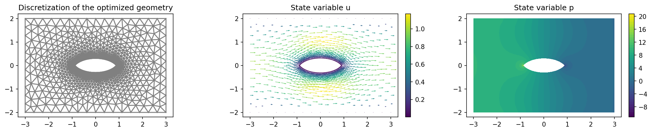
# plt.savefig("./img_eikonal_stiffness.png", dpi=150, bbox_inches="tight")

The results should look like this