cashocs as Solver for Optimal Control Problems#
Problem Formulation#
As a model problem we again consider the one from Distributed Control of a Poisson Problem, but now we do not use cashocs to compute the adjoint equation and derivative of the (reduced) cost functional, but supply these terms ourselves. The optimization problem is given by
(see, e.g., Tröltzsch - Optimal Control of Partial Differential Equations or Hinze, Pinnau, Ulbrich, and Ulbrich - Optimization with PDE constraints).
For the numerical solution of this problem we consider exactly the same setting as in Distributed Control of a Poisson Problem, and most of the code will be identical to this.
Implementation#
The complete python code can be found in the file demo_control_solver.py
and the corresponding config can be found in config.ini.
Recapitulation of Distributed Control of a Poisson Problem#
For using cashocs exclusively as solver, the procedure is very similar to regularly using it, with a few additions after defining the optimization problem. In particular, up to the initialization of the optimization problem, our code is exactly the same as in Distributed Control of a Poisson Problem, i.e., we use
from fenics import *

import cashocs

config = cashocs.load_config("config.ini")
mesh, subdomains, boundaries, dx, ds, dS = cashocs.regular_mesh(25)
V = FunctionSpace(mesh, "CG", 1)

y = Function(V)
p = Function(V)
u = Function(V)

e = inner(grad(y), grad(p)) * dx - u * p * dx

bcs = cashocs.create_dirichlet_bcs(V, Constant(0), boundaries, [1, 2, 3, 4])

y_d = Expression("sin(2*pi*x[0])*sin(2*pi*x[1])", degree=1)
alpha = 1e-6
J = cashocs.IntegralFunctional(
    Constant(0.5) * (y - y_d) * (y - y_d) * dx + Constant(0.5 * alpha) * u * u * dx
)

ocp = cashocs.OptimalControlProblem(e, bcs, J, y, u, p, config=config)
Supplying Custom Adjoint Systems and Derivatives#
When using cashocs as a solver, the user can specify their custom weak forms of the adjoint system and of the derivative of the reduced cost functional. For our optimization problem, the adjoint equation is given by
and the derivative of the cost functional is then given by
Note
For a detailed derivation and discussion of these objects we refer to Tröltzsch - Optimal Control of Partial Differential Equations or Hinze, Pinnau, Ulbrich, and Ulbrich - Optimization with PDE constraints.
To specify that cashocs should use these equations instead of the automatically computed ones, we have the following code. First, we specify the derivative of the reduced cost functional via
dJ = Constant(alpha) * u * TestFunction(V) * dx + p * TestFunction(V) * dx
Afterwards, the weak form for the adjoint system is given by
adjoint_form = (
    inner(grad(p), grad(TestFunction(V))) * dx - (y - y_d) * TestFunction(V) * dx
)
adjoint_bcs = bcs
where we can “recycle” the homogeneous Dirichlet boundary conditions used for the state problem.
For both objects, one has to define them as a single UFL form for cashocs, as with the
state system and cost functional. In particular, the adjoint weak form has to be in
the form of a nonlinear variational problem, so that
fenics.solve(adjoint_form == 0, p, adjoint_bcs) could be used to solve it.
In particular, both forms have to include fenics.TestFunction objects from
the control space and adjoint space, respectively, and must not contain
fenics.TrialFunction objects.
These objects are then supplied to the
OptimalControlProblem via
ocp.supply_custom_forms(dJ, adjoint_form, adjoint_bcs)
Note
One can also specify either the adjoint system or the derivative of the cost
functional, using the methods supply_adjoint_forms or supply_derivatives.
However, this is potentially dangerous, due to the following. The adjoint system
is a linear system, and there is no fixed convention for the sign of the adjoint
state. Hence, supplying, e.g., only the adjoint system, might not be compatible with
the derivative of the cost functional which cashocs computes. In effect, the sign
is specified by the choice of adding or subtracting the PDE constraint from the
cost functional for the definition of a Lagrangian function, which is used to
determine the adjoint system and derivative. cashocs internally uses the convention
that the PDE constraint is added, so that, internally, it computes not the adjoint
state \(p\) as defined by the equations given above, but \(-p\) instead.
Hence, it is recommended to either specify all respective quantities with the
supply_custom_forms
method.
Finally, we can use the solve method
to solve the problem with the line
ocp.solve()
as in Distributed Control of a Poisson Problem.
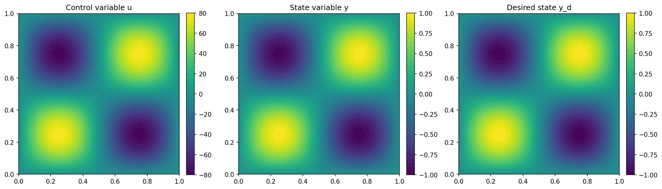
We visualize the results with the lines
import matplotlib.pyplot as plt

plt.figure(figsize=(15, 5))

plt.subplot(1, 3, 1)
fig = plot(u)
plt.colorbar(fig, fraction=0.046, pad=0.04)
plt.title("Control variable u")

plt.subplot(1, 3, 2)
fig = plot(y)
plt.colorbar(fig, fraction=0.046, pad=0.04)
plt.title("State variable y")

plt.subplot(1, 3, 3)
fig = plot(y_d, mesh=mesh)
plt.colorbar(fig, fraction=0.046, pad=0.04)
plt.title("Desired state y_d")

plt.tight_layout()
# plt.savefig('./img_poisson.png', dpi=150, bbox_inches='tight')
The results are, of course, identical to Distributed Control of a Poisson Problem and look as follows
Note
In case we have multiple state equations as in Using Multiple Variables and PDEs, one has to supply ordered lists of adjoint equations and boundary conditions, analogously to the usual procedure for cashocs.
In the case of multiple control variables, the derivatives of the reduced cost functional w.r.t. each of these have to be specified, again using an ordered list.