Topology Optimization with Stokes Flow - Pipe Bend#
Problem Formulation#
In this demo, we consider the topology optimization with Stokes flow, where we aim at finding the optimal shape for a pipe bend. This problem has been investigated previously, e.g., in Blauth and Sturm - Quasi-Newton methods for topology optimization using a level-set method and Sa, Amigo, Novotny, Silva - Topological derivatives applied to fluid flow channel design optimization problems. The problem can be written as follows
Here, \(u\) and \(p\) denote the fluids velocity and pressure, respectively, \(\mu\) is its viscosity. Moreover, \(\alpha\) denotes the viscous resistance or inverse permeability of the material, which is used to distinguish between fluid (where \(\alpha\) is low) and solid (where \(\alpha\) is high). As in the previous demos, e.g. Topology Optimization with Linear Elasticity - Cantilever, \(\alpha\) represents a jumping coefficient between the considered materials, i.e., it is given by \(\alpha_\Omega(x) = \chi_\Omega(x)\alpha_\mathrm{in} + \chi_{\Omega^c}(x) \alpha_\mathrm{out}\), so that \(\Omega\) models our fluid and \(\Omega^c\) models the solid part.
On the outer boundary of the hold-all domain, Dirichlet boundary conditions are specified, indicating, where the fluid enters and exits. Moreover, the goal of the optimization problem is to minimize the energy dissipation of the fluid while achieving a certain volume of the fluid region. For more details on this problem, we refer the reader to Blauth and Sturm - Quasi-Newton methods for topology optimization using a level-set method.
The generalized topological derivative for this problem is given by
Note
We do not specify the adjoint equation here, as this is derived automatically by cashocs. For more details, we refer to Blauth and Sturm - Quasi-Newton methods for topology optimization using a level-set method.
Attention
As in Topology Optimization with a Poisson Equation, there is a minus sign missing in our paper Blauth and Sturm - Quasi-Newton methods for topology optimization using a level-set method. The topological derivative presented here is, in fact, correct.
Implementation#
The complete python code can be found in the file demo_pipe_bend.py,
and the corresponding config can be found in config.ini.
Initialization and Setup#
We start by importing cashocs and FEniCS into our script
from fenics import *
import numpy as np

import cashocs

parameters["dof_ordering_library"] = "Boost"
Next, we load the configuration file for the problem and define the mesh with the lines
cfg = cashocs.load_config("config.ini")
mesh, subdomains, boundaries, dx, ds, dS = cashocs.regular_mesh(25, diagonal="crossed")
Now, we define the finite element spaces for the functions. These are given by a Taylor-Hood space for velocity and pressure variables, a piecewise linear Lagrange space for the level-set function, and a piecewise constant discontinuous Lagrange space for the jumping coefficients.
v_elem = VectorElement("CG", mesh.ufl_cell(), 2)
p_elem = FiniteElement("CG", mesh.ufl_cell(), 1)
V = FunctionSpace(mesh, v_elem * p_elem)
CG1 = FunctionSpace(mesh, "CG", 1)
DG0 = FunctionSpace(mesh, "DG", 0)
Additionally, we define a scalar real
function space (R), which will be used to deal with the volume regularization
of the problem, and a function vol, which represents the current volume of
\(\Omega\), as follows.
R = FunctionSpace(mesh, "R", 0)
vol = Function(R)
Definition of Physical Parameters and Jumping Coefficients#
Next, we define the physical parameters for the problem, including a viscosity of \(\mu = 0.01\) as well as parameters for \(\alpha_\mathrm{in}\) and \(\alpha_\mathrm{out}\)
mu = 1e-2
alpha_in = 2.5 * mu / 1e2**2
alpha_out = 2.5 * mu * 1e2**2
alpha = Function(DG0)
As before, the jumping coefficient \(\alpha\) is represented using a piecewise constant (on each element) function.
Next, the desired volume and the regularization parameter \(\lambda\) are defined, together with the indicator function of \(\Omega\) (see Topology Optimization with Linear Elasticity - Cantilever).
vol_des = assemble(1 * dx) * 0.08 * np.pi
lambd = 1e4
indicator_omega = Function(DG0)
Then, the level-set function is introduced and set to \(\Psi = -1\), so that we use \(\Omega = \mathrm{D}\) as initial guess.
psi = Function(CG1)
psi.vector().vec().set(-1.0)
psi.vector().apply("")
Definition of the State System#
In the following, we define the state and adjoint variables of our problem, in analogy to, e.g., Optimization of an Obstacle in Stokes Flow:
up = Function(V)
u, p = split(up)
vq = Function(V)
v, q = split(vq)
and the weak form of the Stokes system is given by the lines
F = (
    Constant(mu) * inner(grad(u), grad(v)) * dx
    - p * div(v) * dx
    - q * div(u) * dx
    + alpha * dot(u, v) * dx
)
For the Dirichlet boundary conditions, we specify that we have an inflow at the upper left part of the boundary as well as an outflow on the lower right part, with the following expressions.Additionally, we specify the pressure at the point \(x^* = (0,0)\) to obtain uniqueness of the pressure. Altogether, the boundary conditions are specified using the code
v_max = 1e0
v_in = Expression(
    ("(x[1] >= 0.7 && x[1] <= 0.9) ? v_max*(1 - 100*pow(x[1] - 0.8, 2)) : 0.0", "0.0"),
    degree=2,
    v_max=v_max,
)
v_out = Expression(
    ("0.0", "(x[0] >= 0.7 && x[0] <= 0.9) ? -v_max*(1 - 100*pow(x[0] - 0.8, 2)) : 0.0"),
    degree=2,
    v_max=v_max,
)


def pressure_point(x, on_boundary):
    return near(x[0], 0) and near(x[1], 0)


bcs = cashocs.create_dirichlet_bcs(V.sub(0), v_in, boundaries, 1)
bcs += cashocs.create_dirichlet_bcs(V.sub(0), v_out, boundaries, 3)
bcs += cashocs.create_dirichlet_bcs(V.sub(0), Constant((0.0, 0.0)), boundaries, [2, 4])
bcs += [DirichletBC(V.sub(1), Constant(0), pressure_point, method="pointwise")]
Cost Functional and Topological Derivative#
Now, we define the cost functional of our problem as well as its corresponding generalized topological derivative with the lines
J = cashocs.IntegralFunctional(
    Constant(mu) * inner(grad(u), grad(u)) * dx
    + alpha * dot(u, u) * dx
    + Constant(lambd / 2) * pow(vol - Constant(vol_des), 2) * dx
)
dJ_in = Constant(alpha_in - alpha_out) * (dot(u, v) + dot(u, u)) + Constant(lambd) * (
    vol - Constant(vol_des)
)
dJ_out = Constant(alpha_in - alpha_out) * (dot(u, v) + dot(u, u)) + Constant(lambd) * (
    vol - Constant(vol_des)
)
Note
Note, that the second term of the cost functional measures the discrepancy between
the current volume vol of \(\Omega\) and the desired volume. Due to the
update_level_set function, which is defined below, the variable vol holds the
correct value in each iteration.
Note
As in Topology Optimization with a Poisson Equation, the generalized topological derivative for this problem is identical in \(\Omega\) and \(\Omega^c\), which is usually not the case. For this reason, the special structure of the problem can be exploited with the following lines in the configuration file
[TopologyOptimization]
topological_derivative_is_identical = True
As in the previous demos, we have to specify the update routine of the level-set
function update_level_set, which we do as follows:
def update_level_set():
    cashocs.interpolate_levelset_function_to_cells(psi, alpha_in, alpha_out, alpha)
    cashocs.interpolate_levelset_function_to_cells(psi, 1.0, 0.0, indicator_omega)
    vol.vector().vec().set(assemble(indicator_omega * dx))
    vol.vector().apply("")
That is, in the update_level_set function, first the jumping coefficient is updated
with the interpolate_levelset_function_to_cells function.
Then, the indicator function is updated and used to compute the current volume of the
domain, which is written to the variable vol.
Solution of the Topology Optimization Problem#
Finally, we can define the topology optimization problem and solve it via the lines
top = cashocs.TopologyOptimizationProblem(
    F, bcs, J, up, vq, psi, dJ_in, dJ_out, update_level_set, config=cfg
)
top.solve(algorithm="bfgs", rtol=0.0, atol=0.0, angle_tol=5.0, max_iter=500)
Note
For solving this problem, we choose a rather high tolerance (regarding the angle)
of 5 degrees. This means, our optimization algorithm has not yet converged. We do
this to ensure a low running time of the demo. If one wishes, they can run the demo
with angle_tol=1.0 and still recieve a result, however, it may take a while
until this lower tolerance can be reached.
We visualize the result with the code
import matplotlib.pyplot as plt

top.plot_shape()
plt.title("Obtained Pipe Bend Design")
plt.tight_layout()
# plt.savefig("./img_pipe_bend.png", dpi=150, bbox_inches="tight")
and the results looks as follows
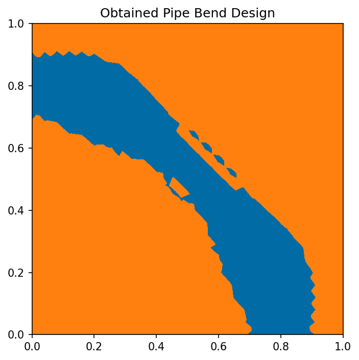
Note
Note that this design is not final due to the following: First, the tolerance for the optimization algorithm is chosen too large, as explained previously. Second, the chosen mesh is rather coarse and, thus, the discretization of the shape is rather coarse, too. These problems can be overcome by using a finer discretization and a lower tolerance.