Optimal Control with Nonlinear PDE Constraints#

Problem Formulation#

In this demo, we take a look at the case of nonlinear PDE constraints for optimization problems. As a model problem, we consider

\[\begin{split} \begin{align} &\min\; J(y,u) = \frac{1}{2} \int_{\Omega} \left( y - y_d \right)^2 \text{ d}x + \frac{\alpha}{2} \int_{\Omega} u^2 \text{ d}x \\ &\text{ subject to } \qquad \begin{alignedat}[t]{2} -\Delta y + c y^3 &= u \quad &&\text{ in } \Omega,\\ y &= 0 \quad &&\text{ on } \Gamma. \end{alignedat} \end{align} \end{split}\]

As this problem has a nonlinear PDE as state constraint, we have to modify the config file slightly. In particular, in the Section StateSystem we have to write

config.ini#

is_linear = False

Note, that is_linear = False works for any problem, as linear equations are just a special case of nonlinear ones, and the corresponding nonlinear solver converges in a single iteration for these. However, in the opposite case, FEniCS will raise an error, so that an actually nonlinear equation cannot be solved using is_linear = True. Also, we briefly recall from Documentation of the Config Files for Optimal Control Problems, that the default behavior is is_linear = False, so that this is not an issue.

Implementation#

The complete python code can be found in the file demo_nonlinear_pdes.py and the corresponding config can be found in config.ini.

Initialization#

Thanks to the high level interface for implementing weak formulations, this problem is tackled almost as easily as the one in Distributed Control of a Poisson Problem. In particular, the entire initialization, up to the definition of the weak form of the PDE constraint, is identical, and we have

from fenics import *

import cashocs

config = cashocs.load_config("config.ini")
mesh, subdomains, boundaries, dx, ds, dS = cashocs.regular_mesh(25)
V = FunctionSpace(mesh, "CG", 1)

y = Function(V)
p = Function(V)
u = Function(V)

For the definition of the state constraints, we use essentially the same syntax as we would use for the problem in FEniCS, i.e., we write

c = Constant(1e2)
e = inner(grad(y), grad(p)) * dx + c * pow(y, 3) * p * dx - u * p * dx

Note

In particular, the only difference between the cashocs implementation of this weak form and the FEniCS one is that, as before, we use fenics.Function objects for both the state and adjoint variables, whereas we would use fenics.Function objects for the state, and fenics.TestFunction for the adjoint variable, which would actually play the role of the test function. Other than that, the syntax is, again, identical to the one of FEniCS.

Finally, the boundary conditions are defined as before

bcs = cashocs.create_dirichlet_bcs(V, Constant(0), boundaries, [1, 2, 3, 4])

Solution of the optimization problem#

To define and solve the optimization problem, we now proceed exactly as in Distributed Control of a Poisson Problem, and use

y_d = Expression("sin(2*pi*x[0])*sin(2*pi*x[1])", degree=1)
alpha = 1e-6
J = cashocs.IntegralFunctional(
    Constant(0.5) * (y - y_d) * (y - y_d) * dx + Constant(0.5 * alpha) * u * u * dx
)

ocp = cashocs.OptimalControlProblem(e, bcs, J, y, u, p, config=config)
ocp.solve()

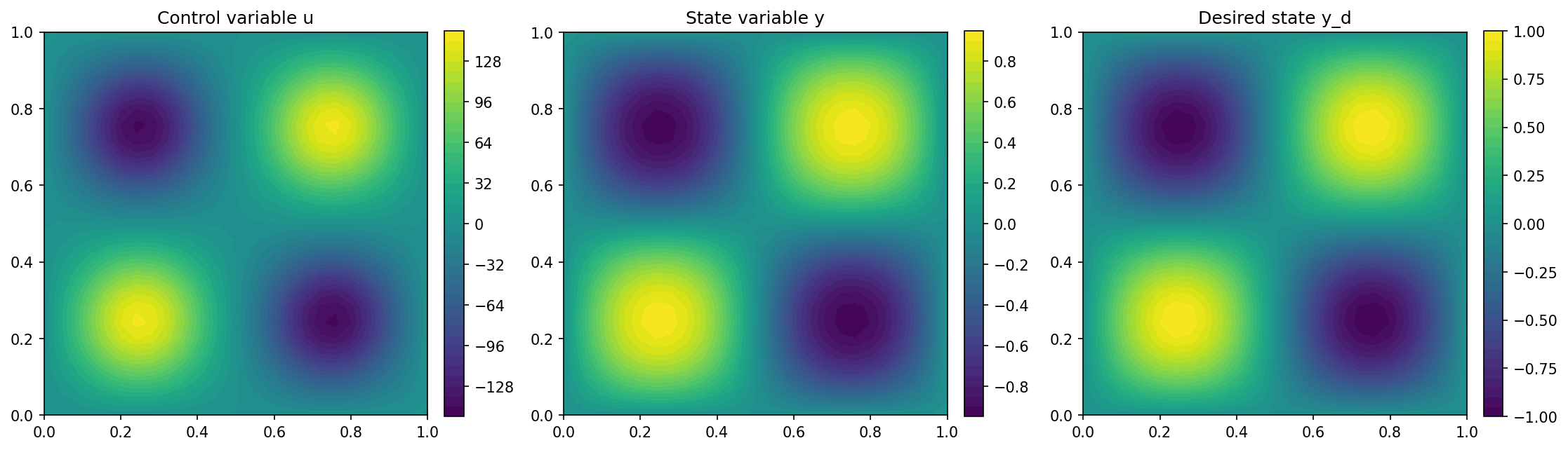
We visualize the results with the lines

import matplotlib.pyplot as plt

plt.figure(figsize=(15, 5))

plt.subplot(1, 3, 1)
fig = plot(u)
plt.colorbar(fig, fraction=0.046, pad=0.04)
plt.title("Control variable u")

plt.subplot(1, 3, 2)
fig = plot(y)
plt.colorbar(fig, fraction=0.046, pad=0.04)
plt.title("State variable y")

plt.subplot(1, 3, 3)
fig = plot(y_d, mesh=mesh)
plt.colorbar(fig, fraction=0.046, pad=0.04)
plt.title("Desired state y_d")

plt.tight_layout()
# plt.savefig('./img_nonlinear_pdes.png', dpi=150, bbox_inches='tight')

and the result looks as follows