Pre- and Post-Callbacks for the optimization#
Problem Formulation#
In this demo we show how one can use the flexibility of cashocs
to “inject” their own code into the optimization, which is carried
out before each solve of the state system (pre_callback) or after each
gradient computation (post_callback). To do so, we investigate the following
problem
In particular, the setting for this demo is very similar to the one of Distributed Control of a Stokes Problem, but here we consider the nonlinear incompressible Navier-Stokes equations.
In the following, we will describe how to solve this problem
using cashocs, where we will use the pre_callback functionality to implement
a homotopy method for solving the Navier-Stokes equations.
Implementation#
The complete python code can be found in the file demo_constraints.py
and the corresponding config can be found in config.ini.
Initialization#
The initial part of the code is nearly identical to the one of Distributed Control of a Stokes Problem, but here we use the Navier-Stokes equations instead of the linear Stokes system
from fenics import *

import cashocs

config = cashocs.load_config("./config.ini")
mesh, subdomains, boundaries, dx, ds, dS = cashocs.regular_mesh(30)

v_elem = VectorElement("CG", mesh.ufl_cell(), 2)
p_elem = FiniteElement("CG", mesh.ufl_cell(), 1)
V = FunctionSpace(mesh, MixedElement([v_elem, p_elem]))
U = VectorFunctionSpace(mesh, "CG", 1)

up = Function(V)
u, p = split(up)
vq = Function(V)
v, q = split(vq)
c = Function(U)

Re = Constant(1e2)

e = (
    inner(grad(u), grad(v)) * dx
    + Constant(Re) * dot(grad(u) * u, v) * dx
    - p * div(v) * dx
    - q * div(u) * dx
    - inner(c, v) * dx
)


def pressure_point(x, on_boundary):
    return near(x[0], 0) and near(x[1], 0)


no_slip_bcs = cashocs.create_dirichlet_bcs(
    V.sub(0), Constant((0, 0)), boundaries, [1, 2, 3]
)
lid_velocity = Expression(("4*x[0]*(1-x[0])", "0.0"), degree=2)
bc_lid = DirichletBC(V.sub(0), lid_velocity, boundaries, 4)
bc_pressure = DirichletBC(V.sub(1), Constant(0), pressure_point, method="pointwise")
bcs = no_slip_bcs + [bc_lid, bc_pressure]

alpha = 1e-5
u_d = Expression(
    (
        "sqrt(pow(x[0], 2) + pow(x[1], 2))*cos(2*pi*x[1])",
        "-sqrt(pow(x[0], 2) + pow(x[1], 2))*sin(2*pi*x[0])",
    ),
    degree=2,
)
J = cashocs.IntegralFunctional(
    Constant(0.5) * inner(u - u_d, u - u_d) * dx
    + Constant(0.5 * alpha) * inner(c, c) * dx
)
Callbacks#
Note, that we have chosen a Reynolds number of Re = 1e2 for this demo.
In order to solve the Navier-Stokes equations for higher Reynolds numbers, it is
often sensible to first solve the equations for a lower Reynolds number and then
use this solution as initial guess for the original high Reynolds number problem.
We can use this procedure in cashocs with its pre_callback functionality.
A pre_callback is a function without arguments, which gets called each time
before solving the state equation. In our case, the pre_callback should
solve the Navier-Stokes equations for a lower Reynolds number, so we define it as
follows
def pre_callback():
    print("Solving low Re Navier-Stokes equations for homotopy.")
    v, q = TestFunctions(V)
    e = (
        inner(grad(u), grad(v)) * dx
        + Constant(Re / 10.0) * dot(grad(u) * u, v) * dx
        - p * div(v) * dx
        - q * div(u) * dx
        - inner(c, v) * dx
    )
    cashocs.snes_solve(e, up, bcs)
where we solve the Navier-Stokes equations with a lower Reynolds number of
Re / 10.0. Later on, we use this function as keyword argument for defining
the optimization problem.
Additionally, cashocs implements the functionality of also performing a pre-defined
action after each gradient computation, given by a so-called post_callback.
In our case, we just want to print a statement so that we can visualize what is
happening. Therefore, we define our post_callback as
def post_callback():
    print("Performing an action after computing the gradient.")
Next, we define the optimization and use the keyword arguments to define the callbacks via
ocp = cashocs.OptimalControlProblem(
    e,
    bcs,
    J,
    up,
    c,
    vq,
    config=config,
    pre_callback=pre_callback,
    post_callback=post_callback,
)
Note
Alternatively, the pre- and post-callbacks can be injected to an already defined optimization problem with the code
ocp.inject_pre_callback(pre_callback)
ocp.inject_post_callback(post_callback)
or, equivalently,
ocp.inject_pre_post_hook(pre_hook, post_hook)
Note
The callback functions are allowed to have one argument. In case an argument is supplied, the callback function is called with the optimization problem itself as an argument during runtime. This allows in-depth manipulation of the optimization algorithms and optimization problems during runtime. This feature should only be used with care!
In the end, we solve the problem with
ocp.solve()
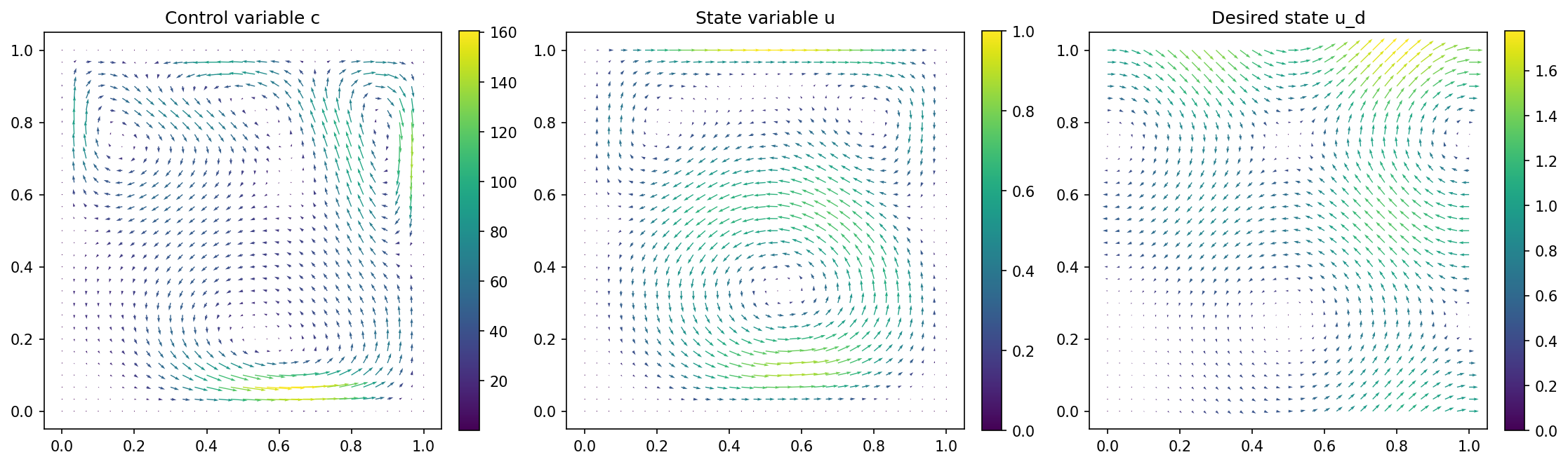
We visualize the results with the lines
u, p = up.split(True)
import matplotlib.pyplot as plt

plt.figure(figsize=(15, 5))

plt.subplot(1, 3, 1)
fig = plot(c)
plt.colorbar(fig, fraction=0.046, pad=0.04)
plt.title("Control variable c")

plt.subplot(1, 3, 2)
fig = plot(u)
plt.colorbar(fig, fraction=0.046, pad=0.04)
plt.title("State variable u")

plt.subplot(1, 3, 3)
fig = plot(u_d, mesh=mesh)
plt.colorbar(fig, fraction=0.046, pad=0.04)
plt.title("Desired state u_d")

plt.tight_layout()
# plt.savefig("./img_pre_post_callbacks.png", dpi=150, bbox_inches="tight")
and the results are given below