Optimal Control with State Constraints#
Problem Formulation#
In this demo we investigate how state constraints can be handled in cashocs. Thanks to the high level interface for solving (control-constrained) optimal control problems, the state constrained case can be treated (approximately) using a Moreau-Yosida regularization, which we show in the following. As model problem, we consider the following one
see, e.g., Hinze, Pinnau, Ulbrich, and Ulbrich - Optimization with PDE constraints.
Moreau-Yosida regularization#
Instead of solving this problem directly, the Moreau-Yosida regularization instead solves a sequence of problems without state constraints which are of the form
for \(\gamma \to +\infty\). We employ a simple homotopy method, and solve the problem for one value of \(\gamma\), and then use this solution as initial guess for the next higher value of \(\gamma\). As initial guess we use the solution of the unconstrained problem. For a detailed discussion of the Moreau-Yosida regularization, we refer the reader to, e.g., Hinze, Pinnau, Ulbrich, and Ulbrich - Optimization with PDE constraints.
Implementation#
The complete python code can be found in the file demo_state_constraints.py
and the corresponding config can be found in config.ini.
The initial guess for the homotopy#
As mentioned earlier, we first solve the unconstrained problem to get an initial guess for the homotopy method. This is done in complete analogy to Distributed Control of a Poisson Problem
from fenics import *
import numpy as np

import cashocs

config = cashocs.load_config("config.ini")
mesh, subdomains, boundaries, dx, ds, dS = cashocs.regular_mesh(25)
V = FunctionSpace(mesh, "CG", 1)

y = Function(V)
p = Function(V)
u = Function(V)

e = inner(grad(y), grad(p)) * dx - u * p * dx
bcs = cashocs.create_dirichlet_bcs(V, Constant(0), boundaries, [1, 2, 3, 4])

y_d = Expression("sin(2*pi*x[0]*x[1])", degree=1)
alpha = 1e-3
J_init_form = (
    Constant(0.5) * (y - y_d) * (y - y_d) * dx + Constant(0.5 * alpha) * u * u * dx
)
J_init = cashocs.IntegralFunctional(J_init_form)
ocp_init = cashocs.OptimalControlProblem(e, bcs, J_init, y, u, p, config=config)
ocp_init.solve()
Note
Cashocs automatically updates the user input during the runtime of the optimization
algorithm. Hence, after the ocp_init.solve() command has returned, the solution is already
stored in u.
The regularized problems#
For the homotopy method with the Moreau-Yosida regularization, we first define the upper bound for the state \(\bar{y}\) and select a sequence of values for \(\gamma\) via
y_bar = 1e-1
gammas = [pow(10, i) for i in np.arange(1, 9, 3)]
Solving the regularized problems is then as simple as writing a for loop
for gamma in gammas:
    J_form = J_init_form + cashocs._utils.moreau_yosida_regularization(
        y, gamma, dx, upper_threshold=y_bar
    )
    J = cashocs.IntegralFunctional(J_form)

    ocp_gamma = cashocs.OptimalControlProblem(e, bcs, J, y, u, p, config=config)
    ocp_gamma.solve()
Here, we use a for loop, define the new cost functional (with the new value of
\(\gamma\)), set up the optimal control problem and solve it, as previously.
Hint
Note that we could have also defined y_bar as a fenics.Function
or fenics.Expression, and the method would have worked exactly the same,
the corresponding object just has to be a valid input for an UFL form.
Note
We could have also defined the Moreau-Yosida regularization of the inequality constraint directly, with the following code
J = cashocs.IntegralFunctional(
    J_init_form
    + Constant(1 / (2 * gamma)) * pow(Max(0, Constant(gamma) * (y - y_bar)), 2) * dx
)
However, this is directly implemented in
cashocs.moreau_yosida_regularization(), which is why we use this function in
the demo.
Validation of the method#
Finally, we perform a post-processing to see whether the state constraint is
(approximately) satisfied. Therefore, we compute the maximum value of y,
and compute the relative error between this and y_bar
y_max = np.max(y.vector()[:])
error = abs(y_max - y_bar) / abs(y_bar) * 100
print("Maximum value of y: " + str(y_max))
print("Relative error between y_max and y_bar: " + str(error) + " %")
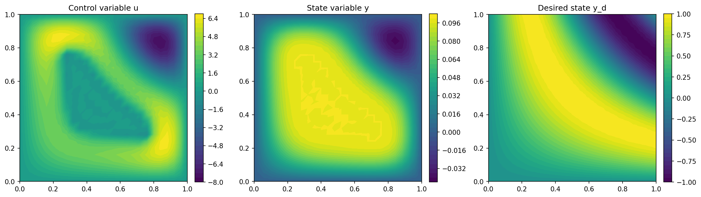
As the error is about 0.01 %, we observe that the regularization indeed works as expected, and this tolerance is sufficiently low for practical applications.
The visualization of the solution is computed with the lines
import matplotlib.pyplot as plt

plt.figure(figsize=(15, 5))

plt.subplot(1, 3, 1)
fig = plot(u)
plt.colorbar(fig, fraction=0.046, pad=0.04)
plt.title("Control variable u")

plt.subplot(1, 3, 2)
fig = plot(y)
plt.colorbar(fig, fraction=0.046, pad=0.04)
plt.title("State variable y")

plt.subplot(1, 3, 3)
fig = plot(y_d, mesh=mesh)
plt.colorbar(fig, fraction=0.046, pad=0.04)
plt.title("Desired state y_d")

plt.tight_layout()
# plt.savefig('./img_state_constraints.png', dpi=150, bbox_inches='tight')
and looks as follows