Scaling of the Cost Functional#
Problem Formulation#
In this demo, we take a look at how cashocs can be used to scale cost functionals, which is particularly useful in case one uses multiple terms to define the cost functional and wants to weight them appropriately, e.g., if there are multiple competing objectives. This demo investigates this problem by considering a slightly modified version of the model shape optimization problem from Shape Optimization with a Poisson Problem, i.e.,
For the initial domain, we use the unit disc \(\Omega = \{ x \in \mathbb{R}^2 \,\mid\, \lvert\lvert x \rvert\rvert_2 < 1 \}\) and the right-hand side \(f\) is given by
Our goal is to choose the parameters \(\alpha\) and \(\beta\) in such a way that the magnitude of the second term is twice as big as the value of the first term for the initial geometry.
Implementation#
The complete python code can be found in the file demo_scaling.py
and the corresponding config can be found in config.ini.
Initialization#
The definition of the PDE constraint is completely identical to the one described in Shape Optimization with a Poisson Problem, which we recall here for the sake of completeness
from fenics import *

import cashocs

config = cashocs.load_config("./config.ini")

mesh, subdomains, boundaries, dx, ds, dS = cashocs.import_mesh("./mesh/mesh.xdmf")

V = FunctionSpace(mesh, "CG", 1)
u = Function(V)
p = Function(V)

x = SpatialCoordinate(mesh)
f = 2.5 * pow(x[0] + 0.4 - pow(x[1], 2), 2) + pow(x[0], 2) + pow(x[1], 2) - 1

e = inner(grad(u), grad(p)) * dx - f * p * dx
bcs = DirichletBC(V, Constant(0), boundaries, 1)
Definition of the Cost Functional#
Our goal is to choose \(\alpha\) and \(\beta\) in such a way that
where \(\Omega_0\) is the intial geometry. Here, we choose the value \(C_1 = 1\) and \(C_2 = 2\) without loss of generality. This would then achieve our goal of having the second term (a volume regularization) being twice as large as the first term in magnitude.
To implement this in cashocs, we do not specify a single UFL form for the cost functional as in all previous demos, instead we supply a list of UFL forms into which we put every single term of the cost functional. These are then scaled automatically by cashocs and then added to obtain the actual cost functional.
Hence, let us first define the individual terms of the cost functional we consider, and place them into a list
J_1 = cashocs.IntegralFunctional(u * dx)
J_2 = cashocs.IntegralFunctional(Constant(1) * dx)
J_list = [J_1, J_2]
Afterwards, we have to create a second list which includes the values that the
terms of J_list should have on the initial geometry
desired_weights = [1, 2]
Finally, these are supplied to the shape optimization problem as follows:
J_list is passed for the usual cost_functional_form
parameter, and desired_weights enters the optimization problem as keyword
argument of the same name, i.e.,
sop = cashocs.ShapeOptimizationProblem(
    e, bcs, J_list, u, p, boundaries, config=config, desired_weights=desired_weights
)
sop.solve()
Note
Since the first term of the cost functional, i.e., \(\int_\Omega u \text{ d}x\), is negative, the initial function value for our choice of scaling is \(-1 + 2 = 1\).
Note
If a cost functional is close to zero for the initial domain, the scaling is
disabled for this term, and instead the respective term is just multiplied
by the corresponding factor in desired_weights. cashocs issues an info
message in this case.
Note
The scaling of the cost functional works completely analogous for optimal control
problems: There, one also has to supply a list of the individual terms of the cost
functional and use the keyword argument desired_weights in order to define
and supply the desired magnitude of the terms for the initial iteration.
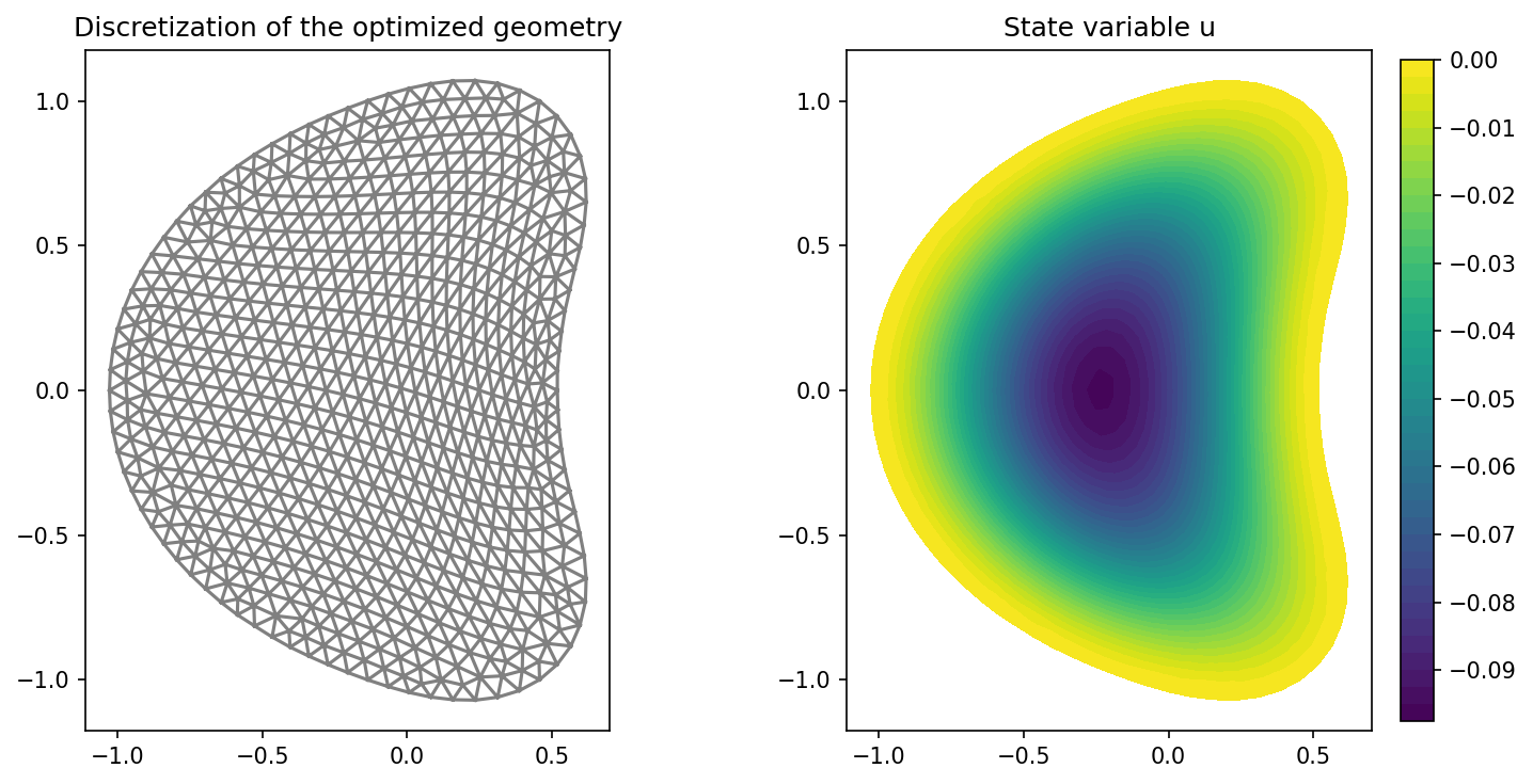
We visualize our results with the code
import matplotlib.pyplot as plt

plt.figure(figsize=(10, 5))

ax_mesh = plt.subplot(1, 2, 1)
fig_mesh = plot(mesh)
plt.title("Discretization of the optimized geometry")

ax_u = plt.subplot(1, 2, 2)
ax_u.set_xlim(ax_mesh.get_xlim())
ax_u.set_ylim(ax_mesh.get_ylim())
fig_u = plot(u)
plt.colorbar(fig_u, fraction=0.046, pad=0.04)
plt.title("State variable u")

plt.tight_layout()
# plt.savefig("./img_scaling.png", dpi=150, bbox_inches="tight")
and obtain the results shown below