Regularization for Shape Optimization Problems#

Problem Formulation#

In this demo, we investigate how we can use regularizations for shape optimization problems in cashocs. For our model problem, we use one similar to the one in Shape Optimization with a Poisson Problem, but which has additional regularization terms, i.e.,

\[\begin{split} \begin{align} \min_\Omega J(u, \Omega) = &\int_\Omega u \text{ d}x + \alpha_\text{vol} \int_\Omega 1 \text{ d}x + \alpha_\text{surf} \int_\Gamma 1 \text{ d}s \\ &+ \frac{\mu_\text{vol}}{2} \left( \int_\Omega 1 \text{ d}x - \text{vol}_\text{des} \right)^2 + \frac{\mu_\text{surf}}{2} \left( \int_\Gamma 1 \text{ d}s - \text{surf}_\text{des} \right)^2 \\ &+ \frac{\mu_\text{curv}}{2} \int_\Gamma \kappa^2 \text{ d}s \\ &\text{subject to} \qquad \begin{alignedat}[t]{2} -\Delta u &= f \quad &&\text{ in } \Omega,\\ u &= 0 \quad &&\text{ on } \Gamma. \end{alignedat} \end{align} \end{split}\]

Here, \(\kappa\) is the mean curvature. For the initial domain, we use the unit disc \(\Omega = \{ x \in \mathbb{R}^2 \,\mid\, \lvert\lvert x \rvert\rvert_2 < 1 \}\) and the right-hand side \(f\) is given by

\[ f(x) = 2.5 \left( x_1 + 0.4 - x_2^2 \right)^2 + x_1^2 + x_2^2 - 1, \]

as in Shape Optimization with a Poisson Problem.

Implementation#

The complete python code can be found in the file demo_regularization.py and the corresponding config can be found in config.ini.

Initialization#

The initial code, including the defition of the PDE constraint, is identical to Shape Optimization with a Poisson Problem, and uses the following code

from fenics import *

import cashocs

config = cashocs.load_config("./config.ini")

mesh, subdomains, boundaries, dx, ds, dS = cashocs.import_mesh("./mesh/mesh.xdmf")

V = FunctionSpace(mesh, "CG", 1)
u = Function(V)
p = Function(V)

x = SpatialCoordinate(mesh)
f = 2.5 * pow(x[0] + 0.4 - pow(x[1], 2), 2) + pow(x[0], 2) + pow(x[1], 2) - 1

e = inner(grad(u), grad(p)) * dx - f * p * dx
bcs = DirichletBC(V, Constant(0), boundaries, 1)

Cost functional and regularization#

The only difference to Shape Optimization with a Poisson Problem comes now, in the definition of the cost functional which includes the additional regularization terms.

The first two summands of the cost functional can then be defined as

alpha_vol = 1e-1
alpha_surf = 1e-1
J = cashocs.IntegralFunctional(
    u * dx + Constant(alpha_vol) * dx + Constant(alpha_surf) * ds
)

The remaining two parts are specified via config.ini, where the following lines are relevant

config.ini#

[Regularization]
factor_volume = 1.0
target_volume = 1.5
use_initial_volume = False
factor_surface = 1.0
target_surface = 4.5
use_initial_surface = False
factor_curvature = 1e-4

This sets the factor \(\mu_\text{vol}\) to 1.0, \(\text{vol}_\text{des}\) to 1.5, \(\mu_\text{surf}\) to 1.0, \(\text{surf}_\text{des}\) to 4.5, and \(\mu_\text{curv}\) to 1e-4. Note that use_initial_volume and use_initial_surface have to be set to False, otherwise the corresponding quantities of the initial geometry would be used instead of the ones prescribed in the config file. The resulting regularization terms are then treated by cashocs, but are, except for these definitions in the config file, invisible for the user.

Note

cashocs can also treat the last two terms directly, making use of the ScalarTrackingFunctional. Therefore, one would use

J_vol = cashocs.ScalarTrackingFunctional(Constant(1.0) * dx, 1.5, weight=1.0)
J_surf = cashocs.ScalarTrackingFunctional(Constant(1.0) * ds, 4.5, weight = 1.0)

However, cashocs is not able to treat the curvature regularization directly, this can only be achieved via the config file option, see the Section Regularization.

Finally, we solve the problem as in Shape Optimization with a Poisson Problem with the lines

sop = cashocs.ShapeOptimizationProblem(e, bcs, J, u, p, boundaries, config=config)
sop.solve()

and we perform a post-processing with the lines

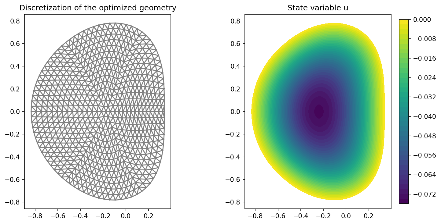
import matplotlib.pyplot as plt

plt.figure(figsize=(10, 5))

ax_mesh = plt.subplot(1, 2, 1)
fig_mesh = plot(mesh)
plt.title("Discretization of the optimized geometry")

ax_u = plt.subplot(1, 2, 2)
ax_u.set_xlim(ax_mesh.get_xlim())
ax_u.set_ylim(ax_mesh.get_ylim())
fig_u = plot(u)
plt.colorbar(fig_u, fraction=0.046, pad=0.04)
plt.title("State variable u")

plt.tight_layout()
# plt.savefig('./img_regularization.png', dpi=150, bbox_inches='tight')

The results should look like this