Sparse Control

Problem Formulation

In this demo, we investigate a possibility for obtaining sparse optimal controls. To do so, we use a sparsity promoting \(L^1\) regularization. Hence, our model problem for this demo is given by

\[\begin{split} \begin{align} &\min\; J(y,u) = \frac{1}{2} \int_{\Omega} \left( y - y_d \right)^2 \text{ d}x + \frac{\alpha}{2} \int_{\Omega} \lvert u \rvert \text{ d}x \\ &\text{ subject to } \qquad \begin{alignedat}[t]{2} -\Delta y &= u \quad &&\text{ in } \Omega,\\ y &= 0 \quad &&\text{ on } \Gamma. \end{alignedat} \end{align} \end{split}\]

This is basically the same problem as in Distributed Control of a Poisson Problem, but the regularization is now not the \(L^2\) norm squared, but just the \(L^1\) norm.

Implementation

The complete python code can be found in the file demo_sparse_control.py and the corresponding config can be found in config.ini.

Initialization

The implementation of this problem is completely analogous to the one of Distributed Control of a Poisson Problem, the only difference is the definition of the cost functional.

from fenics import *

import cashocs

config = cashocs.load_config("config.ini")
mesh, subdomains, boundaries, dx, ds, dS = cashocs.regular_mesh(50)
V = FunctionSpace(mesh, "CG", 1)

y = Function(V)
p = Function(V)
u = Function(V)

e = inner(grad(y), grad(p)) * dx - u * p * dx
bcs = cashocs.create_dirichlet_bcs(V, Constant(0), boundaries, [1, 2, 3, 4])

y_d = Expression("sin(2*pi*x[0])*sin(2*pi*x[1])", degree=1)
alpha = 1e-4

Next, we define the cost function, now using the mentioned \(L^1\) norm for the regularization

J = cashocs.IntegralFunctional(
    Constant(0.5) * (y - y_d) * (y - y_d) * dx + Constant(0.5 * alpha) * abs(u) * dx
)

Note

Note that for the regularization term we now do not use Constant(0.5*alpha)*u*u*dx, which corresponds to the \(L^2(\Omega)\) norm squared, but rather

Constant(0.5 * alpha) * abs(u) * dx

which corresponds to the \(L^1(\Omega)\) norm. Other than that, the code is identical.

We solve the problem analogously to the previous demos

ocp = cashocs.OptimalControlProblem(e, bcs, J, y, u, p, config=config)
ocp.solve()

and we visualize the results with the code

import matplotlib.pyplot as plt

plt.figure(figsize=(15, 5))

plt.subplot(1, 3, 1)
fig = plot(u)
plt.colorbar(fig, fraction=0.046, pad=0.04)
plt.title("Control variable u")

plt.subplot(1, 3, 2)
fig = plot(y)
plt.colorbar(fig, fraction=0.046, pad=0.04)
plt.title("State variable y")

plt.subplot(1, 3, 3)
fig = plot(y_d, mesh=mesh)
plt.colorbar(fig, fraction=0.046, pad=0.04)
plt.title("Desired state y_d")

plt.tight_layout()
# plt.savefig('./img_sparse_control.png', dpi=150, bbox_inches='tight')

which yields the following output

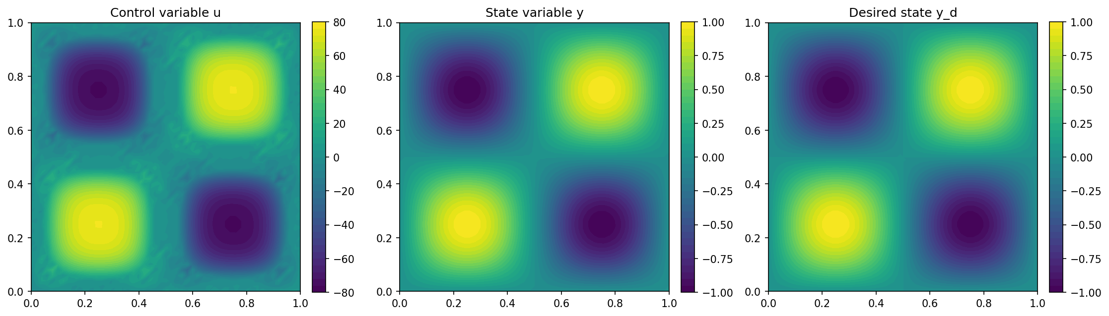
Note

The oscillations in between the peaks for the control variable u are just numerical noise, which comes from the discretization error.