Control Constraints#
Problem Formulation#
In this demo, we take a deeper look at how control constraints can be treated in cashocs. To do so, we investigate the same problem as in Distributed Control of a Poisson Problem, but now with the addition of box constraints for the control variable. This problem reads
(see, e.g., Tröltzsch - Optimal Control of Partial Differential Equations or Hinze, Pinnau, Ulbrich, and Ulbrich - Optimization with PDE constraints.
Here, the functions \(u_a\) and \(u_b\) are \(L^\infty(\Omega)\) functions. As before, we consider as domain the unit square, i.e., \(\Omega = (0, 1)^2\).
Implementation#
The complete python code can be found in the file demo_box_constraints.py
and the corresponding config can be found in config.ini.
Initialization#
The beginning of the script is completely identical to the one of previous example, so we only restate the corresponding code in the following
from fenics import *

import cashocs

config = cashocs.load_config("config.ini")

mesh, subdomains, boundaries, dx, ds, dS = cashocs.regular_mesh(20)
V = FunctionSpace(mesh, "CG", 1)

y = Function(V)
p = Function(V)
u = Function(V)

e = inner(grad(y), grad(p)) * dx - u * p * dx

bcs = cashocs.create_dirichlet_bcs(V, Constant(0), boundaries, [1, 2, 3, 4])

y_d = Expression("sin(2*pi*x[0])*sin(2*pi*x[1])", degree=1)
alpha = 1e-6
J = cashocs.IntegralFunctional(
    Constant(0.5) * (y - y_d) * (y - y_d) * dx + Constant(0.5 * alpha) * u * u * dx
)
Definition of the Control Constraints#
Here, we have nearly everything at hand to define the optimal control problem, the only missing ingredient are the box constraints, which we define now. For the purposes of this example, we consider a linear (in the x-direction) corridor for these constraints, as it highlights the capabilities of cashocs. Hence, we define the lower and upper bounds via
u_a = interpolate(Expression("50*(x[0]-1)", degree=1), V)
u_b = interpolate(Expression("50*x[0]", degree=1), V)
which just corresponds to two functions, generated from fenics.Expression
objects via fenics.interpolate(). These are then put into the list
cc, which models the control constraints, i.e.,
cc = [u_a, u_b]
Note
As an alternative way of specifying the box constraints, one can also use regular float or int objects, in case that they are constant. For example, the constraint that we only want to consider positive value for u, i.e., \(0 \leq u \leq +\infty\) can be realized via
u_a = 0
u_b = float('inf')
cc = [u_a, u_b]
and completely analogous with float('-inf') for no constraint on the lower
bound. Moreover, note that the specification of using either constant float
values and fenics.Function objects can be mixed arbitrarily, so that one
can, e.g., specify a constant value for the upper boundary and use a
fenics.Function on the lower one.
Setup of the optimization problem and its solution#
Now, we can set up the optimal control problem as we did before, using the additional
keyword argument control_constraints into which we put the list
cc, and then solve it via the ocp.solve() method
ocp = cashocs.OptimalControlProblem(
    e, bcs, J, y, u, p, config=config, control_constraints=cc
)
ocp.solve()
To check that the box constraints are actually satisfied by our solution, we perform an assertion
import numpy as np

assert np.all(u_a.vector()[:] <= u.vector()[:]) and np.all(
    u.vector()[:] <= u_b.vector()[:]
)
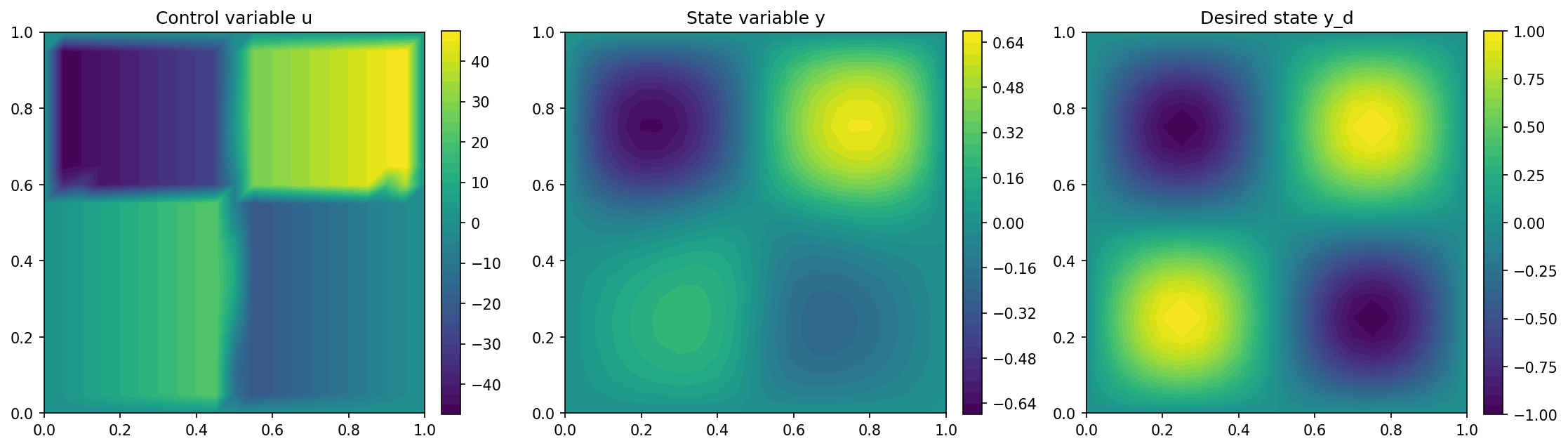
which shows that they are indeed satisfied. The visualization is carried out analogously to before, via
import matplotlib.pyplot as plt

plt.figure(figsize=(15, 5))

plt.subplot(1, 3, 1)
fig = plot(u)
plt.colorbar(fig, fraction=0.046, pad=0.04)
plt.title("Control variable u")

plt.subplot(1, 3, 2)
fig = plot(y)
plt.colorbar(fig, fraction=0.046, pad=0.04)
plt.title("State variable y")

plt.subplot(1, 3, 3)
fig = plot(y_d, mesh=mesh)
plt.colorbar(fig, fraction=0.046, pad=0.04)
plt.title("Desired state y_d")

plt.tight_layout()
# plt.savefig('./img_box_constraints.png', dpi=150, bbox_inches='tight')
and should yield the following output