Custom Scalar Products for Shape Gradient Computation

Problem Formulation

In this demo, we show how to supply a custom bilinear form for the computation of the shape gradient with cashocs. For the sake of simplicity, we again consider our model problem from Shape Optimization with a Poisson Problem, given by

\[\begin{split} \begin{align} &\min_\Omega J(u, \Omega) = \int_\Omega u \text{ d}x \\ &\text{subject to} \qquad \begin{alignedat}[t]{2} -\Delta u &= f \quad &&\text{ in } \Omega,\\ u &= 0 \quad &&\text{ on } \Gamma. \end{alignedat} \end{align} \end{split}\]

For the initial domain, we use the unit disc \(\Omega = \{ x \in \mathbb{R}^2 \,\mid\, \lvert\lvert x \rvert\rvert_2 < 1 \}\) and the right-hand side \(f\) is given by

\[ f(x) = 2.5 \left( x_1 + 0.4 - x_2^2 \right)^2 + x_1^2 + x_2^2 - 1. \]

Implementation

The complete python code can be found in the file demo_custom_scalar_product.py, and the corresponding config can be found in config.ini.

Initialization

The demo program closely follows the one from Shape Optimization with a Poisson Problem, so that up to the definition of the ShapeOptimizationProblem, the code is identical to the one in Shape Optimization with a Poisson Problem, and given by

from fenics import *

import cashocs

config = cashocs.load_config("./config.ini")

mesh, subdomains, boundaries, dx, ds, dS = cashocs.import_mesh("./mesh/mesh.xdmf")

V = FunctionSpace(mesh, "CG", 1)
u = Function(V)
p = Function(V)

x = SpatialCoordinate(mesh)
f = 2.5 * pow(x[0] + 0.4 - pow(x[1], 2), 2) + pow(x[0], 2) + pow(x[1], 2) - 1

e = inner(grad(u), grad(p)) * dx - f * p * dx
bcs = DirichletBC(V, Constant(0), boundaries, 1)

J = cashocs.IntegralFunctional(u * dx)

Definition of the scalar product

To define the scalar product that shall be used for the shape optimization, we can proceed analogously to Neumann Boundary Control and define the corresponding bilinear form in FEniCS. However, note that one has to use a fenics.VectorFunctionSpace with piecewise linear Lagrange elements, i.e., one has to define the corresponding function space as

VCG = VectorFunctionSpace(mesh, "CG", 1)

With this, we can now define the bilinear form as follows

shape_scalar_product = (
    inner((grad(TrialFunction(VCG))), (grad(TestFunction(VCG)))) * dx
    + inner(TrialFunction(VCG), TestFunction(VCG)) * dx
)

Note

Note that we cannot use the formulation

shape_scalar_product = inner((grad(TrialFunction(VCG))), (grad(TestFunction(VCG))))*dx

as this would not yield a coercive bilinear form for this problem. This is due to the fact that the entire boundary of \(\Omega\) is variable. Hence, we actually need this second term.

Finally, we can set up the ShapeOptimizationProblem and solve it with the lines

sop = cashocs.ShapeOptimizationProblem(
    e,
    bcs,
    J,
    u,
    p,
    boundaries,
    config=config,
    shape_scalar_product=shape_scalar_product,
)
sop.solve()

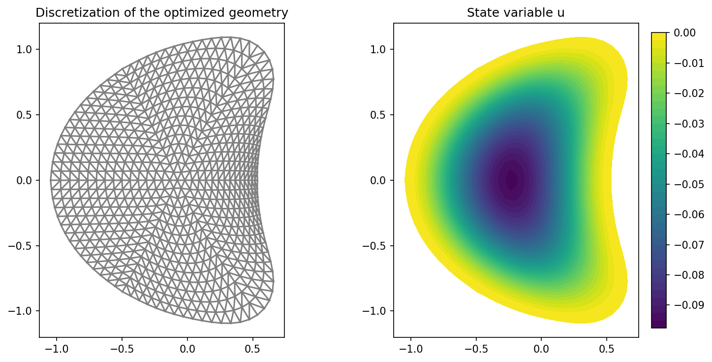
We visualize the result using matplotlib

import matplotlib.pyplot as plt

plt.figure(figsize=(10, 5))

ax_mesh = plt.subplot(1, 2, 1)
fig_mesh = plot(mesh)
plt.title("Discretization of the optimized geometry")

ax_u = plt.subplot(1, 2, 2)
ax_u.set_xlim(ax_mesh.get_xlim())
ax_u.set_ylim(ax_mesh.get_ylim())
fig_u = plot(u)
plt.colorbar(fig_u, fraction=0.046, pad=0.04)
plt.title("State variable u")

plt.tight_layout()
# plt.savefig('./img_custom_scalar_product.png', dpi=150, bbox_inches='tight')

The result of the optimization looks like this