Shape Optimization with a Poisson Problem#

Problem Formulation#

In this demo, we investigate the basics of cashocs for shape optimization problems. As a model problem, we investigate the following one from Etling, Herzog, Loayza, Wachsmuth - First and Second Order Shape Optimization Based on Restricted Mesh Deformations

\[\begin{split} \begin{align} &\min_\Omega J(u, \Omega) = \int_\Omega u \text{ d}x \\ &\text{subject to} \qquad \begin{alignedat}[t]{2} -\Delta u &= f \quad &&\text{ in } \Omega,\\ u &= 0 \quad &&\text{ on } \Gamma. \end{alignedat} \end{align} \end{split}\]

For the initial domain, we use the unit disc \(\Omega = \{ x \in \mathbb{R}^2 \,\mid\, \lvert\lvert x \rvert\rvert_2 < 1 \}\) and the right-hand side \(f\) is given by

\[ f(x) = 2.5 \left( x_1 + 0.4 - x_2^2 \right)^2 + x_1^2 + x_2^2 - 1. \]

Implementation#

The complete python code can be found in the file demo_shape_poisson.py, and the corresponding config can be found in config.ini.

Initialization#

We start the problem by using a wildcard import for FEniCS, and by importing cashocs

from fenics import *

import cashocs

As for the case of optimal control problems, we can specify the verbosity of cashocs with the line

cashocs.set_log_level(cashocs.LogLevel.INFO)

which is documented at cashocs.set_log_level() (cf. Distributed Control of a Poisson Problem).

Similarly to the optimal control case, we also require config files for shape optimization problems in cashocs. A detailed discussion of the config files for shape optimization is given in Documentation of the Config Files for Shape Optimization Problems. We read the config file with the load_config command

config = cashocs.load_config("./config.ini")

Next, we have to define the mesh. We load the mesh (which was previously generated with Gmsh and converted to xdmf with cashocs.convert()

mesh, subdomains, boundaries, dx, ds, dS = cashocs.import_mesh("./mesh/mesh.xdmf")

Note

In config.ini, in the section ShapeGradient, there is the line

config.ini#

[ShapeGradient]
shape_bdry_def = [1]

which specifies that the boundary marked with 1 is deformable. For our example this is exactly what we want, as this means that the entire boundary is variable, due to the fact that the entire boundary is marked by 1 in the Gmsh file. For a detailed documentation we refer to the corresponding documentation of the ShapeGradient section.

After having defined the initial geometry, we define a fenics.FunctionSpace consisting of piecewise linear Lagrange elements via

V = FunctionSpace(mesh, "CG", 1)
u = Function(V)
p = Function(V)

This also defines our state variable \(u\) as u, and the adjoint state \(p\) is given by p.

Note

As remarked in Distributed Control of a Poisson Problem, in classical FEniCS syntax we would use a fenics.TrialFunction for u and a fenics.TestFunction for p. However, for cashocs this must not be the case. Instead, the state and adjoint variables have to be fenics.Function objects.

The right-hand side of the PDE constraint is then defined as

x = SpatialCoordinate(mesh)
f = 2.5 * pow(x[0] + 0.4 - pow(x[1], 2), 2) + pow(x[0], 2) + pow(x[1], 2) - 1

which allows us to define the weak form of the state equation via

e = inner(grad(u), grad(p)) * dx - f * p * dx
bcs = DirichletBC(V, Constant(0), boundaries, 1)

The optimization problem and its solution#

We are now almost done, the only thing left to do is to define the cost functional

J = cashocs.IntegralFunctional(u * dx)

and the shape optimization problem

sop = cashocs.ShapeOptimizationProblem(e, bcs, J, u, p, boundaries, config=config)

This can then be solved in complete analogy to Distributed Control of a Poisson Problem with the sop.solve() command

sop.solve()

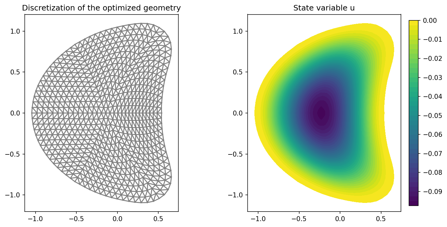
We visualize the result with the following code

import matplotlib.pyplot as plt

plt.figure(figsize=(10, 5))

ax_mesh = plt.subplot(1, 2, 1)
fig_mesh = plot(mesh)
plt.title("Discretization of the optimized geometry")

ax_u = plt.subplot(1, 2, 2)
ax_u.set_xlim(ax_mesh.get_xlim())
ax_u.set_ylim(ax_mesh.get_ylim())
fig_u = plot(u)
plt.colorbar(fig_u, fraction=0.046, pad=0.04)
plt.title("State variable u")

plt.tight_layout()
# plt.savefig('./img_shape_poisson.png', dpi=150, bbox_inches='tight')

and the result should look like this

Note

As in Distributed Control of a Poisson Problem we can specify some keyword arguments for the solve command. If none are given, then the settings from the config file are used, but if some are given, they override the parameters specified in the config file. In particular, these arguments are

algorithm : Specifies which solution algorithm shall be used.

rtol : The relative tolerance for the optimization algorithm.

atol : The absolute tolerance for the optimization algorithm.

max_iter : The maximum amount of iterations that can be carried out.

The possible choices for these parameters are discussed in detail in Section OptimizationRoutine and the documentation of the solve method.

As before, it is not strictly necessary to supply config files to cashocs, but it is very strongly recommended to do so. In case one does not supply a config file, one has to at least specify the solution algorithm in the call to the solve method.