Inverse Problem in Electric Impedance Tomography#
Problem Formulation#
For this demo, we investigate an inverse problem in the setting of electric impedance tomography. It is based on the one used in the preprint Blauth - Nonlinear Conjugate Gradient Methods for PDE Constrained Shape Optimization Based on Steklov-Poincaré-Type Metrics. The problem reads
The setting is as follows. We have an object \(\Omega\) that is located inside another one, \(D \setminus \Omega\). Our goal is to identify the shape of the interior from measurements of the electric potential, denoted by \(u\), on the outer boundary of \(D\), to which we have access. In particular, we consider the case of having several measurements at our disposal, as indicated by the index \(i\). The PDE constraint now models the electric potential in experiment \(i\), namely \(u_i\), which results from an application of the electric current \(f_i\) on the outer boundary \(\partial D\). Our goal of identifying the interior body \(\Omega\) is modeled by the tracking type cost functional, which measures the \(L^2(\Gamma)\) distance between the simulated electric potential \(u_i\) and the measured one, \(m_i\). In particular, note that the outer boundaries, i.e. \(\partial D\) are fixed, and only the internal boundary \(\Gamma = \partial \Omega\) is deformable. For a detailed description of this problem as well as its physical interpretation, we refer to the preprint Blauth - Nonlinear Conjugate Gradient Methods for PDE Constrained Shape Optimization Based on Steklov-Poincaré-Type Metrics.
For our demo, we use as domain the unit square \(D = (0,1)^2\), and the initial geometry of \(\Omega\) is a square inside \(D\). We consider the case of three measurements, so that \(M = 3\), given by
where \(\Gamma^l, \Gamma^r, \Gamma^t, \Gamma^b\) are the left, right, top, and bottom sides of the unit square.
Implementation#
The complete python code can be found in the file
demo_inverse_tomography.py
and the corresponding config can be found in config.ini.
Initialization and generation of synthetic measurements#
We start our code by importing FEniCS and cashocs
from fenics import *

import cashocs
Next, we directly define the sample values of \(\kappa^\text{in}\) and \(\kappa^\text{out}\) since these are needed later on
kappa_out = 1e0
kappa_in = 1e1
In the next part, we generate synthetic measurements, which correspond to \(m_i\).
To do this, we define a function generate_measurements() as follows
def generate_measurements():
    mesh, subdomains, boundaries, dx, ds, dS = cashocs.import_mesh(
        "./mesh/reference.xdmf"
    )

    cg_elem = FiniteElement("CG", mesh.ufl_cell(), 1)
    r_elem = FiniteElement("R", mesh.ufl_cell(), 0)
    V = FunctionSpace(mesh, MixedElement([cg_elem, r_elem]))

    u, c = TrialFunctions(V)
    v, d = TestFunctions(V)

    a = (
        kappa_out * inner(grad(u), grad(v)) * dx(1)
        + kappa_in * inner(grad(u), grad(v)) * dx(2)
        + u * d * ds
        + v * c * ds
    )
    L1 = Constant(1) * v * (ds(3) + ds(4)) + Constant(-1) * v * (ds(1) + ds(2))
    L2 = Constant(1) * v * (ds(3) + ds(2)) + Constant(-1) * v * (ds(1) + ds(4))
    L3 = Constant(1) * v * (ds(3) + ds(1)) + Constant(-1) * v * (ds(2) + ds(4))

    meas1 = Function(V)
    meas2 = Function(V)
    meas3 = Function(V)
    solve(a == L1, meas1)
    solve(a == L2, meas2)
    solve(a == L3, meas3)

    CG1 = V.sub(0).collapse()
    m1 = project(meas1[0], CG1)
    m2 = project(meas2[0], CG1)
    m3 = project(meas3[0], CG1)

    return [m1, m2, m3]
Description of the function
The code executed in generate_measurements() is used to solve the
state problem on a reference domain, given by the mesh ./mesh/reference.xdmf.
This mesh has the domain \(\Omega\) as a circle in the center of the unit
square. To distinguish between these two, we note that \(D \setminus \Omega\)
has the index / marker 1 and that \(\Omega\) has the index / marker 2 in
the corresponding GMSH file, which is then imported into subdomains.
Note, that we have to use a mixed finite element method to incorporate the
integral constraint on the electric potential. The second component of the
corresponding fenics.FunctionSpace V is just a scalar,
one-dimensional, real element. The actual PDE constraint is then given by the part
(
    kappa_out * inner(grad(u), grad(v)) * dx(1)
    + kappa_in * inner(grad(u), grad(v)) * dx(2)
    + ...
)
and the integral constraint is realized with the saddle point formulation
u * d * ds + v * c * ds
The right hand sides L1, L2, and L3 are just given by
the Neumann boundary conditions as specified above.
Finally, these PDEs are then solved via the fenics.solve() command,
and then only the actual solution of the PDE (and not the Lagrange multiplier
for the integral constraint) is returned.
As usual, we load the config into cashocs with the line
config = cashocs.load_config("./config.ini")
Afterwards, we import the mesh into cashocs
mesh, subdomains, boundaries, dx, ds, dS = cashocs.import_mesh("./mesh/mesh.xdmf")
Next, we define the fenics.FunctionSpace object, which consists of
CG1 elements together with a scalar, real element, which acts as a Lagrange multiplier
for the integral constraint
cg_elem = FiniteElement("CG", mesh.ufl_cell(), 1)
r_elem = FiniteElement("R", mesh.ufl_cell(), 0)
V = FunctionSpace(mesh, MixedElement([cg_elem, r_elem]))
Next, we compute the synthetic measurements via
measurement_data = generate_measurements()
In order to ensure that the measurements can be used and stay the same while the mesh undergoes changes in shape optimization, we have to use callbacks, which are explained in full detail in Pre- and Post-Callbacks for the optimization.
measurements = [
    Function(V.sub(0).collapse()),
    Function(V.sub(0).collapse()),
    Function(V.sub(0).collapse()),
]


def pre_callback():
    for i, meas in enumerate(measurements):
        LagrangeInterpolator.interpolate(meas, measurement_data[i])
Here, the function pre_callback is used to interpolate the fixed
measurements to functions on the deformed geometry.
The PDE constraint#
Let us now investigate how the PDE constraint is defined. As we have a mixed finite element problem due to the integral constraint, we proceed similarly to Coupled Problems - Monolithic Approach and define the first state equation with the following lines
uc1 = Function(V)
u1, c1 = split(uc1)
pd1 = Function(V)
p1, d1 = split(pd1)
e1 = (
    kappa_out * inner(grad(u1), grad(p1)) * dx(1)
    + kappa_in * inner(grad(u1), grad(p1)) * dx(2)
    + u1 * d1 * ds
    + p1 * c1 * ds
    - Constant(1) * p1 * (ds(3) + ds(4))
    - Constant(-1) * p1 * (ds(1) + ds(2))
)
The remaining two experiments are defined completely analogously:
uc2 = Function(V)
u2, c2 = split(uc2)
pd2 = Function(V)
p2, d2 = split(pd2)
e2 = (
    kappa_out * inner(grad(u2), grad(p2)) * dx(1)
    + kappa_in * inner(grad(u2), grad(p2)) * dx(2)
    + u2 * d2 * ds
    + p2 * c2 * ds
    - Constant(1) * p2 * (ds(3) + ds(2))
    - Constant(-1) * p2 * (ds(1) + ds(4))
)

uc3 = Function(V)
u3, c3 = split(uc3)
pd3 = Function(V)
p3, d3 = split(pd3)
e3 = (
    kappa_out * inner(grad(u3), grad(p3)) * dx(1)
    + kappa_in * inner(grad(u3), grad(p3)) * dx(2)
    + u3 * d3 * ds
    + p3 * c3 * ds
    - Constant(1) * p3 * (ds(3) + ds(1))
    - Constant(-1) * p3 * (ds(2) + ds(4))
)
Finally, we group together the state equations as well as the state and adjoint variables to (ordered) lists, as in Using Multiple Variables and PDEs
e = [e1, e2, e3]
u = [uc1, uc2, uc3]
p = [pd1, pd2, pd3]
Since the problem only has Neumann boundary conditions, we use
bcs = [[], [], []]
to specify this.
The shape optimization problem#
The cost functional is then defined by first creating the individual summands, and then adding them to a list:
J1 = cashocs.IntegralFunctional(Constant(0.5) * pow(u1 - measurements[0], 2) * ds)
J2 = cashocs.IntegralFunctional(Constant(0.5) * pow(u2 - measurements[1], 2) * ds)
J3 = cashocs.IntegralFunctional(Constant(0.5) * pow(u3 - measurements[2], 2) * ds)

J = [J1, J2, J3]
where we use a coefficient of \(\nu_i = 1\) for all cases.
Before we can define the shape optimization properly, we have to take a look at the config file to specify which boundaries are fixed, and which are deformable. There, we have the following lines
[ShapeGradient]
shape_bdry_def = []
shape_bdry_fix = [1, 2, 3, 4]
Note, that the boundaries 1, 2, 3, 4 are the sides of the unit square, as
defined in the .geo file for the geometry (located in the ./mesh/ directory), and
they are fixed due to the problem definition (recall that \(\partial D\) is fixed).
However, at the first glance it seems that there is no deformable boundary. This
is, however, wrong. In fact, there is still an internal boundary, namely \(\Gamma\),
which is not specified here, and which is, thus, deformable (this is the default
behavior).
Warning
As stated in Documentation of the Config Files for Shape Optimization Problems, we have to use the config file setting
use_pull_back = False
This is due to the fact that the measurements are defined / computed on a different
mesh / geometry than the remaining objects, and FEniCS is not able to do some
computations in this case. However, note that the cost functional is posed on
\(\partial D\) only, which is fixed anyway. Hence, the deformation field
vanishes there, and the corresponding diffeomorphism, which maps between the
deformed and original domain, is just the identity mapping. In particular,
no material derivatives are needed for the measurements, which is why it
is safe to use use_pull_back = False for this particular problem.
The shape optimization problem can now be created as in Shape Optimization with a Poisson Problem and can be solved as easily, with the commands
sop = cashocs.ShapeOptimizationProblem(e, bcs, J, u, p, boundaries, config=config)
sop.inject_pre_callback(pre_callback)
sop.solve()
We perform a post-processing of the results with the lines
import matplotlib.pyplot as plt

DG0 = FunctionSpace(mesh, "DG", 0)
plt.figure(figsize=(10, 5))

result = Function(DG0)
a_post = TrialFunction(DG0) * TestFunction(DG0) * dx
L_post = Constant(1) * TestFunction(DG0) * dx(1) + Constant(2) * TestFunction(DG0) * dx(
    2
)
solve(a_post == L_post, result)

ax_result = plt.subplot(1, 2, 2)
fig_result = plot(result)
plt.title("Optimized Geometry")

mesh_initial, _, _, dx, _, _ = cashocs.import_mesh("./mesh/mesh.xdmf")
DG0 = FunctionSpace(mesh_initial, "DG", 0)
initial = Function(DG0)
a_post = TrialFunction(DG0) * TestFunction(DG0) * dx
L_post = Constant(1) * TestFunction(DG0) * dx(1) + Constant(2) * TestFunction(DG0) * dx(
    2
)
solve(a_post == L_post, initial)

ax_initial = plt.subplot(1, 2, 1)
fig_initial = plot(initial)
plt.title("Initial Geometry")

plt.tight_layout()
# plt.savefig('./img_inverse_tomography.png', dpi=150, bbox_inches='tight')
and the results should look like this
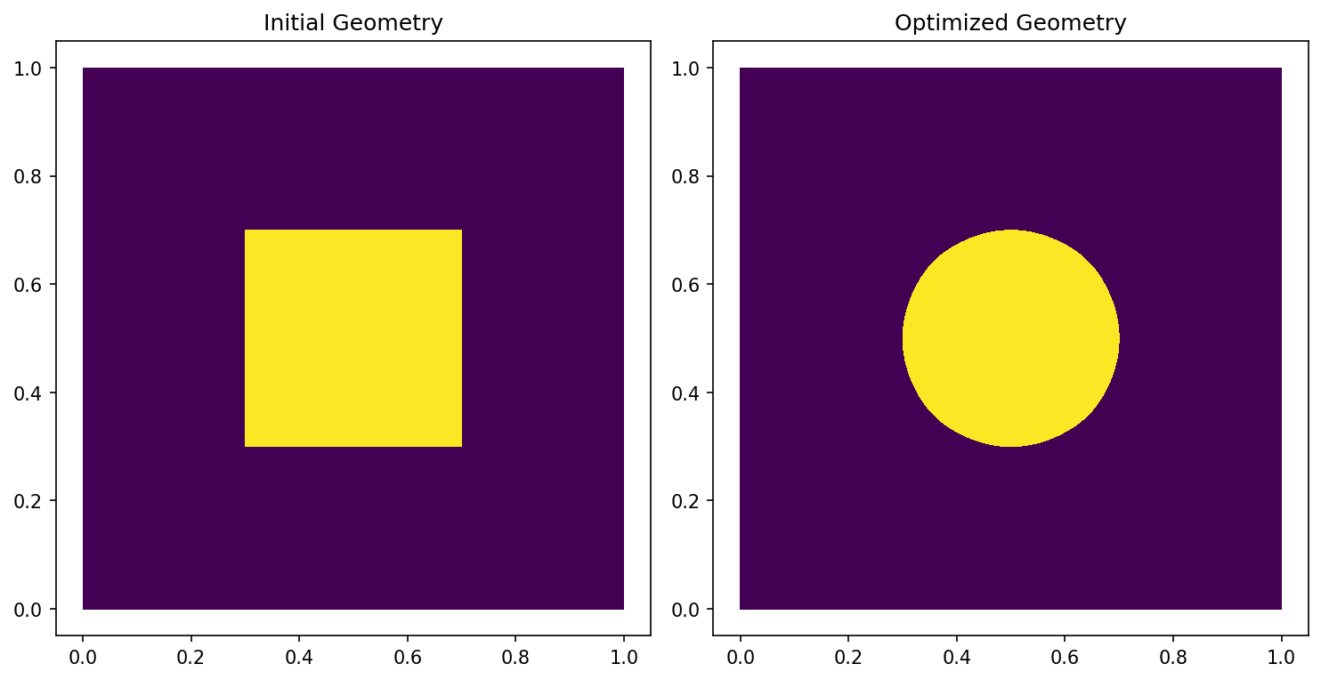
and we observe that we are indeed able to identify the shape of the circle which was used to create the measurements.