Shape Optimization with the p-Laplacian

Problem Formulation

In this demo, we take a look at yet another possibility to compute the shape gradient and to use this method for solving shape optimization problems. Here, we investigate the approach of Müller, Kühl, Siebenborn, Deckelnick, Hinze, and Rung and use the \(p\)-Laplacian in order to compute the shape gradient. As a model problem, we consider the following one, as in Shape Optimization with a Poisson Problem:

\[\begin{split} \begin{align} &\min_\Omega J(u, \Omega) = \int_\Omega u \text{ d}x \\ &\text{subject to} \qquad \begin{alignedat}[t]{2} -\Delta u &= f \quad &&\text{ in } \Omega,\\ u &= 0 \quad &&\text{ on } \Gamma. \end{alignedat} \end{align} \end{split}\]

For the initial domain, we use the unit disc \(\Omega = \{ x \in \mathbb{R}^2 \,\mid\, \lvert\lvert x \rvert\rvert_2 < 1 \}\) and the right-hand side \(f\) is given by

\[ f(x) = 2.5 \left( x_1 + 0.4 - x_2^2 \right)^2 + x_1^2 + x_2^2 - 1. \]

Implementation

The complete python code can be found in the file demo_p_laplacian.py and the corresponding config can be found in config.ini.

Source Code

The python source code for this example is completely identical to the one in Shape Optimization with a Poisson Problem, and we will repeat the code at the end of the tutorial. The only changes occur in the configuration file, which we cover below.

Changes in the Configuration File

All the relevant changes appear in the ShapeGradient Section of the config file, where we now add the following three lines

config.ini

[ShapeGradient]
use_p_laplacian = True
p_laplacian_power = 10
p_laplacian_stabilization = 0.0

Here, use_p_laplacian is a boolean flag which indicates that we want to override the default behavior and use the \(p\) Laplacian to compute the shape gradient instead of linear elasticity. In particular, this means that we solve the following equation to determine the shape gradient \(\mathcal{G}\)

\[\begin{split} \begin{aligned} &\text{Find } \mathcal{G} \text{ such that } \\ &\qquad \int_\Omega \mu \left( \nabla \mathcal{G} : \nabla \mathcal{G} \right)^{\frac{p-2}{2}} \nabla \mathcal{G} : \nabla \mathcal{V} + \delta \mathcal{G} \cdot \mathcal{V} \text{ d}x = dJ(\Omega)[\mathcal{V}] \\ &\text{for all } \mathcal{V}. \end{aligned} \end{split}\]

Here, \(dJ(\Omega)[\mathcal{V}]\) is the shape derivative. The parameter \(p\) is defined via the config file parameter p_laplacian_power, and is 10 for this example. Finally, it is possible to use a stabilized formulation of the \(p\)-Laplacian equation shown above, where the stabilization parameter is determined via the config line parameter p_laplacian_stabilization, which should be small (e.g. in the order of 1e-3). Moreover, \(\mu\) is the stiffness parameter, which can be specified via the config file parameters mu_def and mu_fixed and works as usually (cf. Shape Optimization with a Poisson Problem:). Finally, we have added the possibility to use the damping parameter \(\delta\), which is specified via the config file parameter damping_factor, also in the Section ShapeGradient.

Note

Note that the \(p\)-Laplace methods are only meant to work with the gradient descent method. Other methods, such as BFGS or NCG methods, might be able to work on certain problems, but you might encounter strange behavior of the methods.

Finally, the code for the demo looks as follows

from fenics import *

import cashocs

cashocs.set_log_level(cashocs.LogLevel.INFO)

config = cashocs.load_config("./config.ini")

mesh, subdomains, boundaries, dx, ds, dS = cashocs.import_mesh("./mesh/mesh.xdmf")

V = FunctionSpace(mesh, "CG", 1)
u = Function(V)
p = Function(V)

x = SpatialCoordinate(mesh)
f = 2.5 * pow(x[0] + 0.4 - pow(x[1], 2), 2) + pow(x[0], 2) + pow(x[1], 2) - 1

e = inner(grad(u), grad(p)) * dx - f * p * dx
bcs = DirichletBC(V, Constant(0), boundaries, 1)

J = cashocs.IntegralFunctional(u * dx)

sop = cashocs.ShapeOptimizationProblem(e, bcs, J, u, p, boundaries, config=config)
sop.solve()

import matplotlib.pyplot as plt

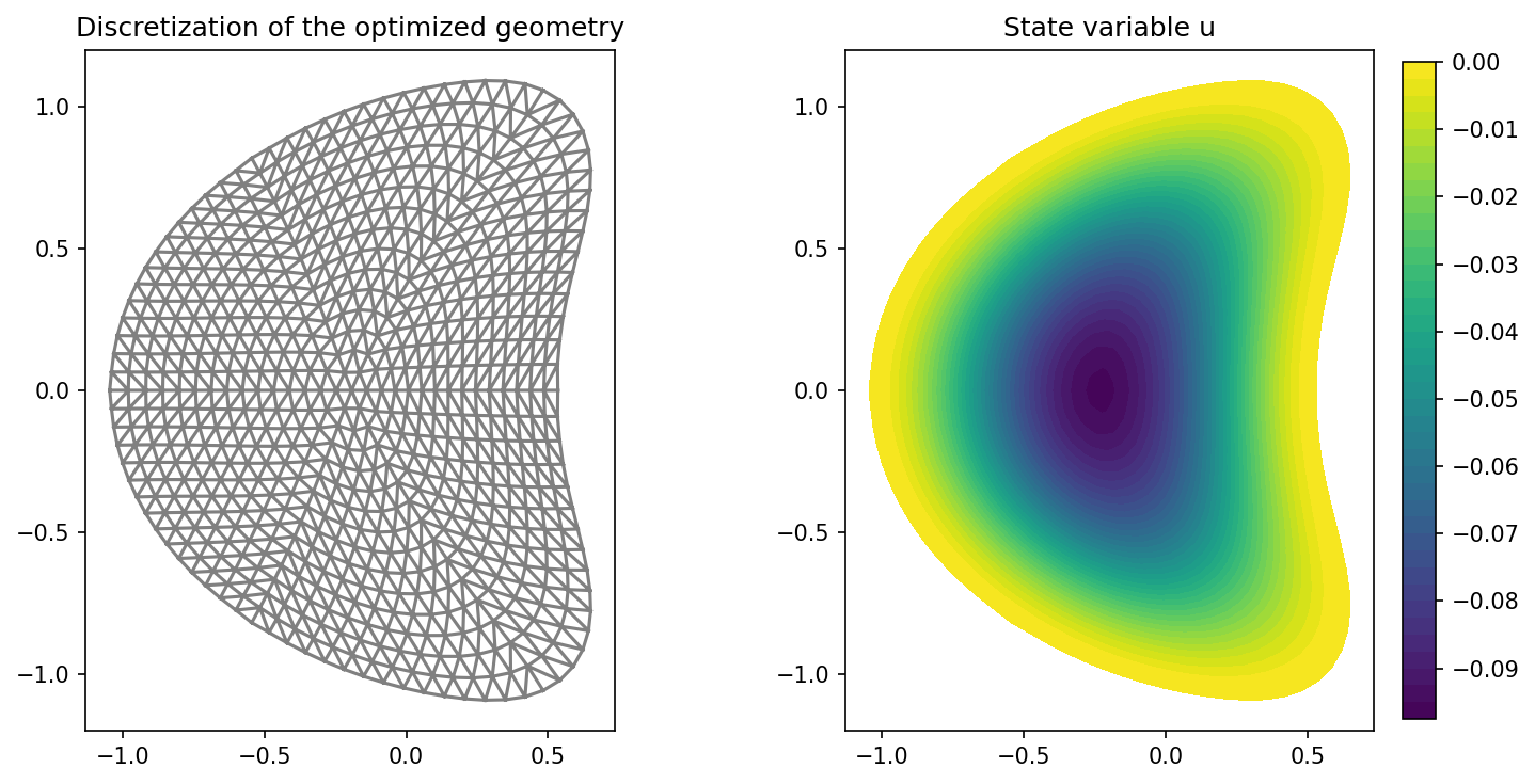
plt.figure(figsize=(10, 5))

ax_mesh = plt.subplot(1, 2, 1)
fig_mesh = plot(mesh)
plt.title("Discretization of the optimized geometry")

ax_u = plt.subplot(1, 2, 2)
ax_u.set_xlim(ax_mesh.get_xlim())
ax_u.set_ylim(ax_mesh.get_ylim())
fig_u = plot(u)
plt.colorbar(fig_u, fraction=0.046, pad=0.04)
plt.title("State variable u")

plt.tight_layout()
# plt.savefig("./img_p_laplacian.png", dpi=150, bbox_inches="tight")

and the results of the optimization look like this