Neumann Boundary Control

Problem Formulation

In this demo we investigate an optimal control problem with a Neumann type boundary control. This problem reads

\[\begin{split} \begin{align} &\min\; J(y,u) = \frac{1}{2} \int_{\Omega} \left( y - y_d \right)^2 \text{ d}x + \frac{\alpha}{2} \int_{\Gamma} u^2 \text{ d}s \\ &\text{ subject to } \qquad \begin{alignedat}[t]{2} -\Delta y + y &= 0 \quad &&\text{ in } \Omega,\\ n\cdot \nabla y &= u \quad &&\text{ on } \Gamma. \end{alignedat} \end{align} \end{split}\]

(see, e.g., Tröltzsch - Optimal Control of Partial Differential Equations or Hinze, Pinnau, Ulbrich, and Ulbrich - Optimization with PDE constraints. Note that we cannot use a simple Poisson equation as constraint since this would not be compatible with the boundary conditions (i.e. not well-posed).

Implementation

The complete python code can be found in the file demo_neumann_control.py and the corresponding config can be found in config.ini.

Initialization

Initially, the code is again identical to the previous ones (see Distributed Control of a Poisson Problem and Control Constraints), i.e., we have

from fenics import *

import cashocs

config = cashocs.load_config("config.ini")

mesh, subdomains, boundaries, dx, ds, dS = cashocs.regular_mesh(25)
V = FunctionSpace(mesh, "CG", 1)

y = Function(V)
p = Function(V)
u = Function(V)

Definition of the state equation

Now, the definition of the state problem obviously differs from the previous two examples, and we use

e = inner(grad(y), grad(p)) * dx + y * p * dx - u * p * ds

which directly puts the Neumann boundary condition into the weak form. For this problem, we do not have Dirichlet boundary conditions, so that we use

bcs = []

Hint

Alternatively, we could have also used

bcs = None

Definition of the cost functional

The definition of the cost functional is nearly identical to before, only the integration measure for the regularization term changes, so that we have

y_d = Expression("sin(2*pi*x[0])*sin(2*pi*x[1])", degree=1)
alpha = 1e-6
J = cashocs.IntegralFunctional(
    Constant(0.5) * (y - y_d) * (y - y_d) * dx + Constant(0.5 * alpha) * u * u * ds
)

As the default Hilbert space for a control is \(L^2(\Omega)\), we now also have to change this, to accommodate for the fact that the control variable u now lies in the space \(L^2(\Gamma)\), i.e., it is only defined on the boundary. This is done by defining the scalar product of the corresponding Hilbert space, which we do with

scalar_product = TrialFunction(V) * TestFunction(V) * ds

The scalar_product always has to be a symmetric, coercive and continuous bilinear form, so that it induces an actual scalar product on the corresponding space.

Note

This means, that we could also define an alternative scalar product for Distributed Control of a Poisson Problem, using the space \(H^1(\Omega)\) instead of \(L^2(\Omega)\) with the following

scalar_product = (
    inner(grad(TrialFunction(V)), grad(TestFunction(V))) * dx
    + TrialFunction(V) * TestFunction(V) * dx
)

This allows a great amount of flexibility in the choice of the control space.

Setup of the optimization problem and its solution

With this, we can now define the optimal control problem with the additional keyword argument riesz_scalar_products and solve it with the ocp.solve() command

ocp = cashocs.OptimalControlProblem(
    e, bcs, J, y, u, p, config=config, riesz_scalar_products=scalar_product
)
ocp.solve()

Hence, in order to treat boundary control problems, the corresponding weak forms have to be modified accordingly, and one has to adapt the scalar products used to determine the gradients.

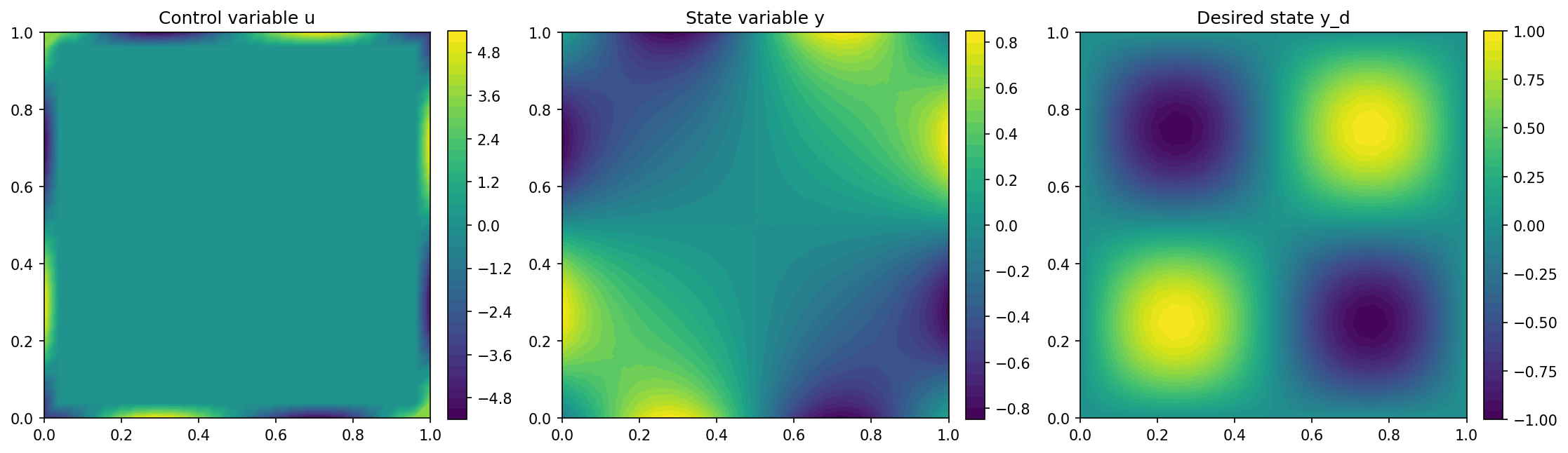
We visualize the results with the lines

import matplotlib.pyplot as plt

plt.figure(figsize=(15, 5))

plt.subplot(1, 3, 1)
fig = plot(u)
plt.colorbar(fig, fraction=0.046, pad=0.04)
plt.title("Control variable u")

plt.subplot(1, 3, 2)
fig = plot(y)
plt.colorbar(fig, fraction=0.046, pad=0.04)
plt.title("State variable y")

plt.subplot(1, 3, 3)
fig = plot(y_d, mesh=mesh)
plt.colorbar(fig, fraction=0.046, pad=0.04)
plt.title("Desired state y_d")

plt.tight_layout()
# plt.savefig('./img_neumann_control.png', dpi=150, bbox_inches='tight')

and the output should look like this