Coupled Problems - Monolithic Approach#
Problem Formulation#
In this demo we show how cashocs can be used with a coupled PDE constraint. For this demo, we consider a monolithic approach, whereas we investigate an approach based on a Picard iteration in Coupled Problems - Picard Iteration.
As model example, we consider the following problem
In constrast to Using Multiple Variables and PDEs, the system is now two-way coupled. To solve it, we employ a mixed finite element method in this demo.
Implementation#
The complete python code can be found in the file demo_monolithic_problems.py
and the corresponding config can be found in config.ini.
Initialization#
The initialization for this example works as before, i.e., we use
from fenics import *

import cashocs

config = cashocs.load_config("config.ini")
mesh, subdomains, boundaries, dx, ds, dS = cashocs.regular_mesh(50)
For the mixed finite element method we have to define a
fenics.MixedFunctionSpace, via
elem_1 = FiniteElement("CG", mesh.ufl_cell(), 1)
elem_2 = FiniteElement("CG", mesh.ufl_cell(), 1)
V = FunctionSpace(mesh, MixedElement([elem_1, elem_2]))
The control variables get their own fenics.FunctionSpace
U = FunctionSpace(mesh, "CG", 1)
Then, the state and adjoint variables state and adjoint are
defined
state = Function(V)
adjoint = Function(V)
As these are part of a fenics.MixedFunctionSpace, we can access their
individual components by
y, z = split(state)
p, q = split(adjoint)
Similarly to Using Multiple Variables and PDEs, p is the adjoint state
corresponding to y, and q is the one corresponding to z.
We then define the control variables as
u = Function(U)
v = Function(U)
controls = [u, v]
Note, that we directly put the control variables u and v into a
list controls, which implies that u is the first component of the
control variable, and v the second one.
Hint
An alternative way of specifying the controls would be to reuse the mixed function space and use
controls = Function(V)
u, v = split(controls)
Although this formulation is slightly different (it uses a
fenics.Function for the controls, and not a list) the de-facto behavior of
both methods is completely identical, just the interpretation is slightly different
(since the individual components of the fenics.FunctionSpace V
are also CG1 functions).
Definition of the mixed weak form#
Next, we define the mixed weak form. To do so, we first define the first equation and its Dirichlet boundary conditions
e_y = inner(grad(y), grad(p)) * dx + z * p * dx - u * p * dx
bcs_y = cashocs.create_dirichlet_bcs(V.sub(0), Constant(0), boundaries, [1, 2, 3, 4])
and, in analogy, the second state equation
e_z = inner(grad(z), grad(q)) * dx + y * q * dx - v * q * dx
bcs_z = cashocs.create_dirichlet_bcs(V.sub(1), Constant(0), boundaries, [1, 2, 3, 4])
To arrive at the mixed weak form of the entire syste, we have to add the state equations and Dirichlet boundary conditions
e = e_y + e_z
bcs = bcs_y + bcs_z
Note, that we can only have one state equation as we also have only a single state
variable state, and the number of state variables and state equations has
to coincide, and the same is true for the boundary conditions, where also just a
single list is required.
Defintion of the optimization problem#
The cost functional can be specified in analogy to the one of Using Multiple Variables and PDEs
y_d = Expression("sin(2*pi*x[0])*sin(2*pi*x[1])", degree=1)
z_d = Expression("sin(4*pi*x[0])*sin(4*pi*x[1])", degree=1)
alpha = 1e-6
beta = 1e-6
J = cashocs.IntegralFunctional(
    Constant(0.5) * (y - y_d) * (y - y_d) * dx
    + Constant(0.5) * (z - z_d) * (z - z_d) * dx
    + Constant(0.5 * alpha) * u * u * dx
    + Constant(0.5 * beta) * v * v * dx
)
Finally, we can set up the optimization problem and solve it
optimization_problem = cashocs.OptimalControlProblem(
    e, bcs, J, state, controls, adjoint, config=config
)
optimization_problem.solve()
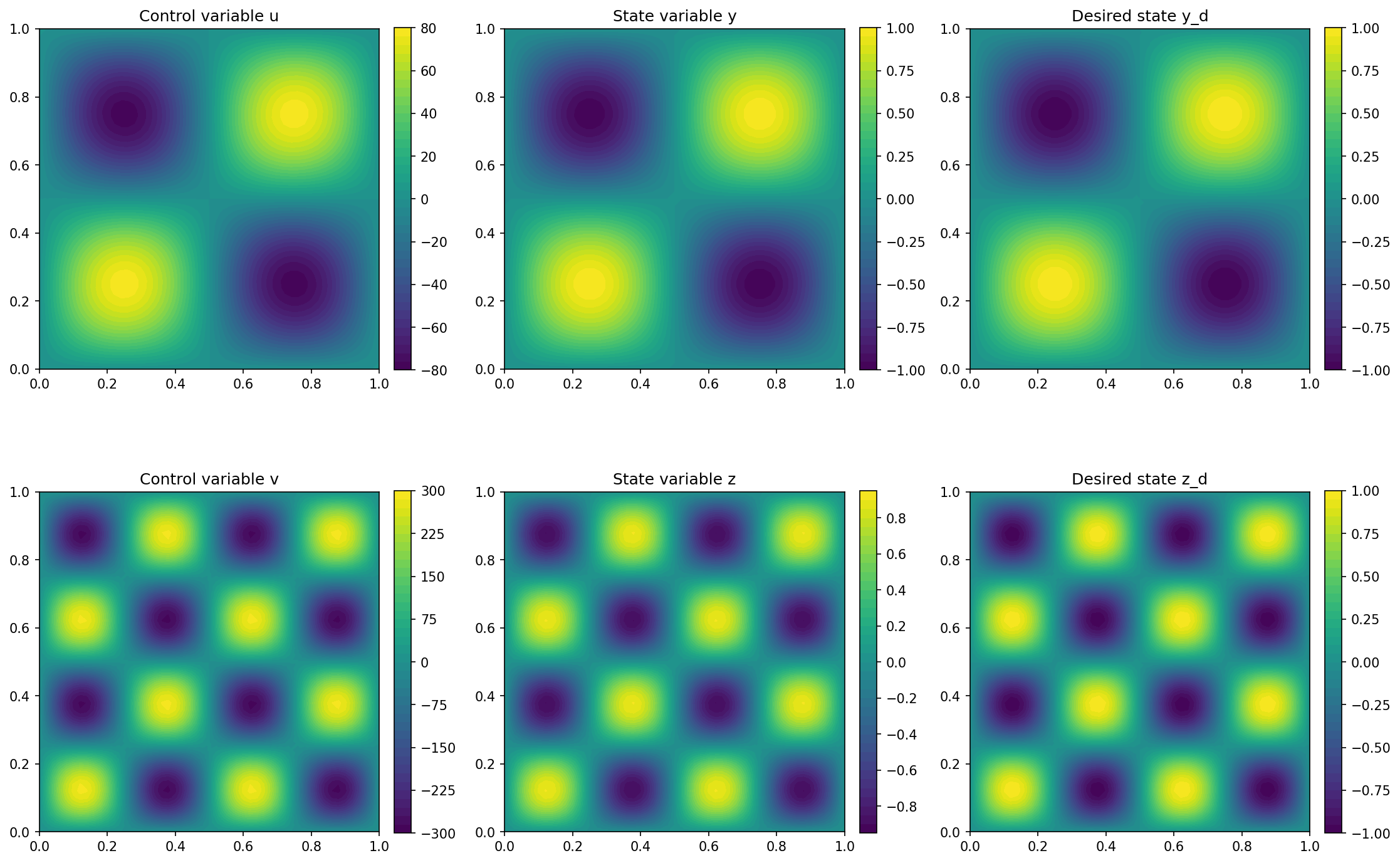
We visualize the result with the code
y, z = state.split(True)
import matplotlib.pyplot as plt

plt.figure(figsize=(15, 10))

plt.subplot(2, 3, 1)
fig = plot(u)
plt.colorbar(fig, fraction=0.046, pad=0.04)
plt.title("Control variable u")

plt.subplot(2, 3, 2)
fig = plot(y)
plt.colorbar(fig, fraction=0.046, pad=0.04)
plt.title("State variable y")

plt.subplot(2, 3, 3)
fig = plot(y_d, mesh=mesh)
plt.colorbar(fig, fraction=0.046, pad=0.04)
plt.title("Desired state y_d")

plt.subplot(2, 3, 4)
fig = plot(v)
plt.colorbar(fig, fraction=0.046, pad=0.04)
plt.title("Control variable v")

plt.subplot(2, 3, 5)
fig = plot(z)
plt.colorbar(fig, fraction=0.046, pad=0.04)
plt.title("State variable z")

plt.subplot(2, 3, 6)
fig = plot(z_d, mesh=mesh)
plt.colorbar(fig, fraction=0.046, pad=0.04)
plt.title("Desired state z_d")

plt.tight_layout()
# plt.savefig('./img_monolithic_problems.png', dpi=150, bbox_inches='tight')
so that the output should look like this