Iterative Solvers for State and Adjoint Systems#
Problem Formulation#
cashocs is also capable of using iterative solvers through the linear algebra backend PETSc. In this demo we show how this can be used. For the sake of simplicitiy, we consider the same setting as in Distributed Control of a Poisson Problem, i.e.
(see, e.g., Tröltzsch - Optimal Control of Partial Differential Equations or Hinze, Pinnau, Ulbrich, and Ulbrich - Optimization with PDE constraints.
It is well-known, that the state problem, when discretized using a classical, conforming Ritz-Galerkin method, gives rise to a linear system with a symmetric and positive definite matrix. We use these properties in this demo by solving the state system with the conjugate gradient method. Moreover, the adjoint system is also a Poisson problem with right-hand side \(y - y_d\), and so also gives rise to a symmetric and positive definite system, for which we also employ an iterative solver.
Implementation#
The complete python code can be found in the file demo_iterative_solvers.py
and the corresponding config can be found in config.ini.
Initialization#
The initialization works exactly as in Distributed Control of a Poisson Problem
from fenics import *

import cashocs

config = cashocs.load_config("config.ini")
mesh, subdomains, boundaries, dx, ds, dS = cashocs.regular_mesh(50)
V = FunctionSpace(mesh, "CG", 1)

y = Function(V)
p = Function(V)
u = Function(V)

e = inner(grad(y), grad(p)) * dx - u * p * dx
bcs = cashocs.create_dirichlet_bcs(V, Constant(0), boundaries, [1, 2, 3, 4])
Definition of the iterative solvers#
The options for the state and adjoint systems are defined as follows. For the state system we have
ksp_options = {
    "ksp_type": "cg",
    "pc_type": "hypre",
    "pc_hypre_type": "boomeramg",
    "ksp_rtol": 1e-10,
    "ksp_atol": 1e-13,
    "ksp_max_it": 100,
}
This is a list of lists, where the inner ones have either 1 or 2 entries, which correspond to the command line options for PETSc. For a detailed documentation of the possibilities, we refer to the PETSc documentation. Of particular interest are the pages for the Krylov solvers and Preconditioners. The relevant options for the command line are described under “Options Database Keys”.
Note
For example, the first line
"ksp_type": "cg",
can be found in KSPSetType and the corresponding options are shown under KSPTYPE. Here, we see that the above line corresponds to using the conjugate gradient method as krylov solver. The following two lines
"pc_type": "hypre",
"pc_hypre_type": "boomeramg",
specify that we use the algebraic multigrid preconditioner BOOMERAMG from HYPRE. This is documented in PCSetType, PCTYPE, and PCHYPRE. Finally, the last three lines
"ksp_rtol": 1e-10,
"ksp_atol": 1e-13,
"ksp_max_it": 100,
specify that we use a relative tolerance of 1e-10, an absolute one of 1e-13, and at most 100 iterations for each solve of the linear system, cf. KSPSetTolerances.
Coming from the first optimize, then discretize view point, it is not required that the adjoint system should be solved exactly the same as the state system. This is why we can also define PETSc options for the adjoint system, which we do with
adjoint_ksp_options = {
    "ksp_type": "minres",
    "pc_type": "jacobi",
    "ksp_rtol": 1e-6,
    "ksp_atol": 1e-15,
}
As can be seen, we now use a completely different solver, namely MINRES (the minimal residual method) with a jacobi preconditioner. Finally, the tolerances for the adjoint solver can also be rather different from the ones of the state system, as is shown here.
Hint
To verify that the options indeed are used, one can supply the option
'ksp_view': None,
which shows the detailed settings of the solvers, and also
'ksp_monitor_true_residual': None,
which prints the residual of the method over its iterations.
For multiple state and adjoint systems, one can proceed analogously to Using Multiple Variables and PDEs, and one has to create a such a list of options for each component, and then put them into an additional list.
With these definitions, we can now proceed as in Distributed Control of a Poisson Problem and solve the optimization problem with
y_d = Expression("sin(2*pi*x[0])*sin(2*pi*x[1])", degree=1)
alpha = 1e-6
J = cashocs.IntegralFunctional(
    Constant(0.5) * (y - y_d) * (y - y_d) * dx + Constant(0.5 * alpha) * u * u * dx
)

ocp = cashocs.OptimalControlProblem(
    e,
    bcs,
    J,
    y,
    u,
    p,
    config=config,
    ksp_options=ksp_options,
    adjoint_ksp_options=adjoint_ksp_options,
)
ocp.solve()
Note
Note, that if the ksp_options and adjoint_ksp_options are not
passed to the OptimalControlProblem or
None, which is the default value of these keyword parameters, then the
direct solver MUMPS is used. Moreover, if one wants to use identical options for state
and adjoint systems, then only the ksp_options have to be passed. This is
because adjoint_ksp_options always mirrors the ksp_options in case that the
input is None for adjoint_ksp_options.
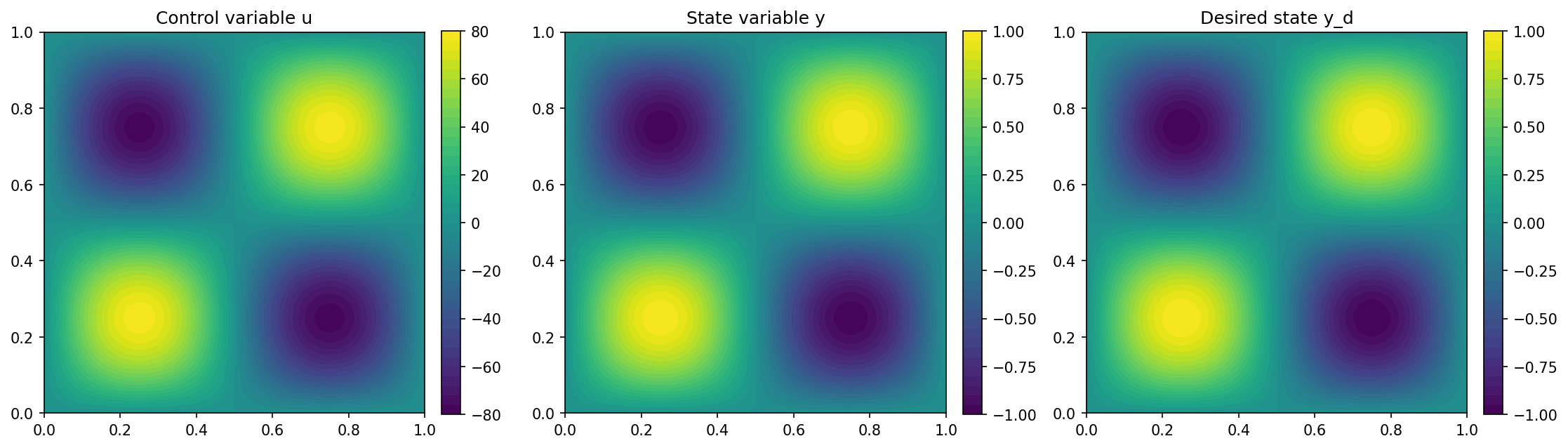
We visualize the results of the optimization with the lines
import matplotlib.pyplot as plt

plt.figure(figsize=(15, 5))

plt.subplot(1, 3, 1)
fig = plot(u)
plt.colorbar(fig, fraction=0.046, pad=0.04)
plt.title("Control variable u")

plt.subplot(1, 3, 2)
fig = plot(y)
plt.colorbar(fig, fraction=0.046, pad=0.04)
plt.title("State variable y")

plt.subplot(1, 3, 3)
fig = plot(y_d, mesh=mesh)
plt.colorbar(fig, fraction=0.046, pad=0.04)
plt.title("Desired state y_d")

plt.tight_layout()
# plt.savefig('./img_iterative_solvers.png', dpi=150, bbox_inches='tight')
and the result should look like this