Topology Optimization with Linear Elasticity - Cantilever#
Problem Formulation#
In this demo, we consider the topology optimization of linear elastic structures, using the well-known cantilever example, which has been investigated, e.g., in Blauth and Sturm - Quasi-Newton methods for topology optimization using a level-set method and Amstutz and Andrä - A new algorithm for topology optimization using a level-set method. Our goal is to minimize the compliance of a linear elastic material, which can be formulated via the topology optimization problem
Here, \(u\) is the deformation of a linear elastic material, \(\sigma(u) = 2 \mu e(u) + \lambda \text{tr}e(u)I\) is Hooke’s tensor, where \(e(u) = \frac{1}{2}\left( \nabla u + (\nabla u)^T \right)\) is the symmetric gradient. The coefficients \(\mu\) and \(\lambda\) are the Lamé parameters which satisfy \(\mu \geq 0\) and \(2\mu + d \lambda > 0\), where \(d\) is the dimension of the problem. As in Topology Optimization with a Poisson Equation, the coefficient \(\alpha_\Omega\) is given by \(\alpha_\Omega(x) = \chi_\Omega(x)\alpha_\mathrm{in} + \chi_{\Omega^c}(x) \alpha_\mathrm{out}\), and it models the elasticity of the material. We note that the term \(\gamma \lvert \Omega\rvert\) is used to penalize too large domains \(\Omega\) so that not the trivial solution \(\Omega = \mathrm{D}\) is found. On the Dirichlet boundary \(\Gamma_D\), the material is fixed, and at the Neumann boundary \(\Gamma_N\) a load \(g\) is applied.
Note that the generalized topological derivative for this problem is given by
where \(r_\mathrm{in} = \frac{\alpha_\mathrm{out}}{\alpha_\mathrm{in}}\), \(r_\mathrm{out} = \frac{\alpha_\mathrm{in}}{\alpha_\mathrm{out}}\), and \(\kappa = \frac{\lambda + 3\mu}{\lambda + \mu}\).
Note
In the following, we consider only two-dimensional problems. For this case of plane stress, the Lamé parameters are given by \(\mu = \frac{E}{2(1+\nu)}\) and \(\lambda = \frac{2\mu \lambda^*}{\lambda^* + 2\mu}\), where \(\lambda^* = \frac{E\nu}{(1+\nu)(1-2\nu)}\) and \(E\) and \(\nu\) denote the Young’s modulus and Poisson’s ratio of the material, respectively.
Implementation#
The complete python code can be found in the file demo_cantilever.py,
and the corresponding config can be found in config.ini.
Initialization and Setup#
As with all other demos, we start by importing FEniCS and cashocs.
from fenics import *

import cashocs
Next, we load the configuration file of the problem with the line
cfg = cashocs.load_config("config.ini")
Following this, we define the computational domain, using the built-in
regular_mesh function, so that our hold-all domain
is given by
\(\mathrm{D} = (0,2) \times (0,1)\).
mesh, subdomains, boundaries, dx, ds, dS = cashocs.regular_mesh(
    32, length_x=2.0, diagonal="crossed"
)
Next up, we define the function spaces for the problems. The solution of the state (and adjoint) systems lives in a vector function space of piecewise linear Lagrange elements, which is defined with
V = VectorFunctionSpace(mesh, "CG", 1)
We also define scalar piecewise linear Lagrange elements (the CG1 space) and
piecewise constant discontinuous Lagrange elements (the DG0 space) in the following.
The CG1 space is needed to represent the level-set function and the DG0 space
is used to treat the jumping coefficients.
CG1 = FunctionSpace(mesh, "CG", 1)
DG0 = FunctionSpace(mesh, "DG", 0)
Now, we define the level-set function which represents our geometry (see the previous demo), and we initialize it with \(\Psi = -1\), so that \(\Omega = \mathrm{D}\) as initial guess.
psi = Function(CG1)
psi.vector().vec().set(-1.0)
psi.vector().apply("")
Definition of the Material Parameters#
In the following lines, we define the physical and numerical parameters for the material and optimization problem. First, the penalty parameter \(\gamma\) is defined as
gamma = 100.0
Next, we define the Lamé parameters for the material, using a Young’s modulus of \(E = 1\) and Poisson’s ratio of \(\nu = 0.3\)
E = 1.0
nu = 0.3
mu = E / (2.0 * (1.0 + nu))
lambd_star = E * nu / ((1.0 + nu) * (1.0 - 2.0 * nu))
lambd = 2 * mu * lambd_star / (lambd_star + 2.0 * mu)
Finally, the parameters \(\alpha_\mathrm{in}\) and \(\alpha_\mathrm{out}\) are defined as
alpha_in = 1.0
alpha_out = 1e-3
alpha = Function(DG0)
which models the presence of material in \(\Omega\) as well as the absence thereof in \(\Omega^c\). As before, \(\alpha\) is a jumping coefficient, so that we define a piecewise constant FEM function which will represent it later.
As we also need to take care of the volume \(\lvert \Omega \rvert\), we define a indicator function for the domain \(\Omega\), which is, as the jumping coefficient represented by a piecewise constant function.
indicator_omega = Function(DG0)
Note
As cells cut by the level-set function will recieve averaged values in these piecewise constant functions, the integral of the indicator function even gives us the exact volume of \(\Omega\).
Definition of the State System#
In the following, we define two python functions which return Hooke’s tensor and the symmetrized gradient
def eps(u):
    return Constant(0.5) * (grad(u) + grad(u).T)


def sigma(u):
    return Constant(2.0 * mu) * eps(u) + Constant(lambd) * tr(eps(u)) * Identity(2)
For the load applied to the system we use a unitary point load at (2, 0.5), i.e., in
the middle of the outer rightmost boundary. To do so, a Dirac-Delta function can be
defined via a FEniCS UserExpression as follows.
class Delta(UserExpression):
    def __init__(self, *args, **kwargs):
        super().__init__(*args, **kwargs)

    def eval(self, values, x):
        if near(x[0], 2.0) and near(x[1], 0.5):
            values[0] = 3.0 / mesh.hmax()
        else:
            values[0] = 0.0

    def value_shape(self):
        return ()
We use this definition to define the point load as follows
delta = Delta(degree=2)
g = delta * Constant((0.0, -1.0))
Next, we define the state and adjoint variables \(u\) and \(v\)
u = Function(V)
v = Function(V)
as well as the state system, the linear elasticity equations
F = alpha * inner(sigma(u), eps(v)) * dx - dot(g, v) * ds(2)
which is supplied with boundary conditions of the form
bcs = cashocs.create_dirichlet_bcs(V, Constant((0.0, 0.0)), boundaries, 1)
Setup of the Cost Functional and Topological Derivative#
To define the topology optimization problem, we first define the cost functional of the problem, given by
J = cashocs.IntegralFunctional(
    alpha * inner(sigma(u), eps(u)) * dx + Constant(gamma) * indicator_omega * dx
)
Note
As stated before, the integration of the function indiciator_omega gives the exact
volume of \(\Omega\), so that the regularization term can be written as above.
Finally, as stated previously, we have to specify the generalized topological derivative of the problem, which has been derived above. This is done with the lines
kappa = (lambd + 3.0 * mu) / (lambd + mu)
r_in = alpha_out / alpha_in
r_out = alpha_in / alpha_out

dJ_in = (
    Constant(alpha_in * (r_in - 1.0) / (kappa * r_in + 1.0) * (kappa + 1.0) / 2.0)
    * (
        Constant(2.0) * inner(sigma(u), eps(u))
        + Constant((r_in - 1.0) * (kappa - 2.0) / (kappa + 2 * r_in - 1.0))
        * tr(sigma(u))
        * tr(eps(u))
    )
) + Constant(gamma)
dJ_out = (
    Constant(-alpha_out * (r_out - 1.0) / (kappa * r_out + 1.0) * (kappa + 1.0) / 2.0)
    * (
        Constant(2.0) * inner(sigma(u), eps(u))
        + Constant((r_out - 1.0) * (kappa - 2.0) / (kappa + 2 * r_out - 1.0))
        * tr(sigma(u))
        * tr(eps(u))
    )
) + Constant(gamma)
As in Topology Optimization with a Poisson Equation, we now only have to specify what needs to happen
when the level-set function is updated, i.e., when the geometry changes. Of course,
the jumping coefficient \(\alpha\) needs to be updated with the
interpolate_levelset_function_to_cells function, but so does the
indicator function of the geometry. This is specified in the following function.
def update_level_set():
    cashocs.interpolate_levelset_function_to_cells(psi, alpha_in, alpha_out, alpha)
    cashocs.interpolate_levelset_function_to_cells(psi, 1.0, 0.0, indicator_omega)
Note
As we want indicator_omega to be the indicator function of \(\Omega\), the
above call makes sure that it is \(1\) inside \(\Omega\) and \(0\) outside
of it, representing a proper indicator function.
Definition and Solution of the Topology Optimization Problem#
Now, all that is left to do is to define the
TopologyOptimizationProblem and
solve it with its solve method.
top = cashocs.TopologyOptimizationProblem(
    F, bcs, J, u, v, psi, dJ_in, dJ_out, update_level_set, config=cfg
)
top.solve(algorithm="bfgs", rtol=0.0, atol=0.0, angle_tol=1.5, max_iter=250)
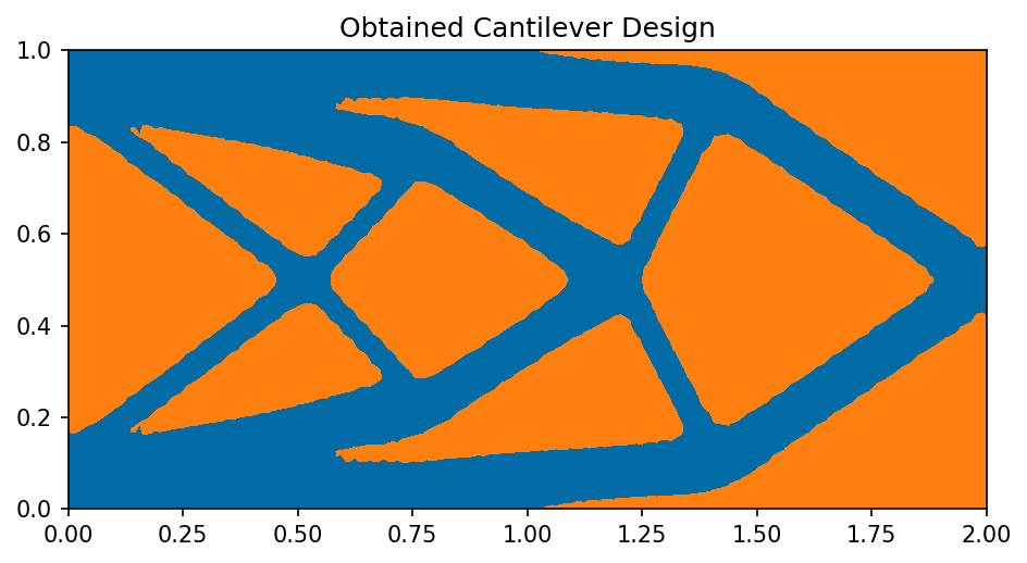
As before, we can visualize the result using the following code
import matplotlib.pyplot as plt

top.plot_shape()
plt.title("Obtained Cantilever Design")
plt.tight_layout()
# plt.savefig("./img_cantilever.png", dpi=150, bbox_inches="tight")
and the result looks like this