Space Mapping Shape Optimization - Semilinear Transmission Problem#
Problem Formulation#
In this demo we detail the space mapping capabilities of cashocs. The space mapping technique is used to optimize a fine (detailed, costly, expensive) model with the help of a coarse (cheaper, approximate) one. In particular, only coarse model optimizations are required, whereas for the fine model we only require simulations. This makes the technique very attractive when using commercial solvers for the fine model, while using, e.g., cashocs, as solver for the coarse model optimization problem. For an overview over the space mapping technique, we refer the reader, e.g., to Bakr, Bandler, Madsen, Sondergaard - An Introduction to the Space Mapping Technique and Echeverria and Hemker - Space mapping and defect correction. For a detailed description of the methods in the context of shape optimization, we refer to Blauth - Space Mapping for PDE Constrained Shape Optimization.
For this example, we consider the one investigated numerically in Section 4.2 of Blauth - Space Mapping for PDE Constrained Shape Optimization. Let us now state the semi linear transmission which we want to solve. It is given by
Here, \(\alpha\) is given by \(\alpha(x) = \chi_\Omega(x) \alpha_1 + (1 - \chi_\Omega(x)) \alpha_2\) and \(f\) is given by \(f(x) = \chi_\Omega(x) f_1 + (1 - \chi_\Omega(x)) f_2\). The above optimization problem plays the role of the fine model. Note that the difficulty of this problem comes from the nonlinear term in the state equation, which makes the PDE constraint harder to solver than a linear equation. Therefore, we want to use an approximate model which is easier to solve. Our coarse model for this problem is given by
The difference between the fine and the coarse model optimization problems is now only the difference in the PDE constraints, i.e., the coarse model problem is the same as the fine model with \(\beta = 0\). This can also be interpreted as linearization of the fine model around \(u = 0\).
Note
Note that we also need a misalignment function in order to match the fine and coarse model outputs. For this problem, a natural choice is to use the misalignment function
This leads to a parameter extraction step in which the following subproblem has to be solved
Implementation#
The complete python code can be found in the file
demo_space_mapping_semilinear_transmission.py
and the corresponding config can be found in config.ini.
The coarse model#
We start our description of the space mapping technqiue with the implementation of the
coarse model. For this, we can use standard cashocs syntax, with the difference that
we will not put the cost functional, etc., into a
cashocs.ShapeOptimizationProblem, but we will use a
CoarseModel for the
coarse model.
As usual, we begin the script with importing cashocs and fenics
import os

from fenics import *

import cashocs
Next, we define the space mapping module we are using in the line
space_mapping = cashocs.space_mapping.shape_optimization
and, further, we decrease the verbosity of cashocs so that we can see only the output of the space mapping routine
cashocs.set_log_level(cashocs.log.ERROR)
Finally, we define the path to the current directory (where the script is located) via
dir = os.path.dirname(os.path.realpath(__file__))
Next, we define some model parameters and load the configuration file for the problem
alpha_1 = 1.0
alpha_2 = 10.0
f_1 = 1.0
f_2 = 10.0
beta = 100.0
cfg = cashocs.load_config("config.ini")
In the next step, we define our desired state \(u_\mathrm{des}\) as solution of the fine model state constraint with a given geometry \(\Omega\)
def create_desired_state(alpha_1, alpha_2, beta, f_1, f_2):
    mesh, subdomains, boundaries, dx, ds, dS = cashocs.import_mesh(
        "./mesh/reference.xdmf"
    )
    V = FunctionSpace(mesh, "CG", 1)
    u = Function(V)
    v = TestFunction(V)
    F = (
        Constant(alpha_1) * dot(grad(u), grad(v)) * dx(1)
        + Constant(alpha_2) * dot(grad(u), grad(v)) * dx(2)
        + Constant(beta) * pow(u, 3) * v * dx
        - Constant(f_1) * v * dx(1)
        - Constant(f_2) * v * dx(2)
    )
    bcs = cashocs.create_dirichlet_bcs(V, Constant(0.0), boundaries, [1, 2, 3, 4])
    cashocs.snes_solve(F, u, bcs)

    return u


u_des_fixed = create_desired_state(alpha_1, alpha_2, beta, f_1, f_2)
Here, u_des_fixed plays the role of the fixed desired state, which is given
on a different mesh than the one we consider for the optimization later on.
Note
As u_des_fixed is given on another mesh and represents a fixed state, it has to be
re-interpolated during each iteration of the optimization algorithms. This is due to
the fact that, otherwise, it would be moved along with the mesh / geometry that is to
be optimized and then become distorted. Therefore, a re-interpolation has to happen.
Now, we can define the coarse model, in analogy to Shape Optimization with a Poisson Problem
mesh, subdomains, boundaries, dx, ds, dS = cashocs.import_mesh("./mesh/mesh.xdmf")
V = FunctionSpace(mesh, "CG", 1)

u = Function(V)
p = Function(V)
u_des = Function(V)
F = (
    Constant(alpha_1) * dot(grad(u), grad(p)) * dx(1)
    + Constant(alpha_2) * dot(grad(u), grad(p)) * dx(2)
    - Constant(f_1) * p * dx(1)
    - Constant(f_2) * p * dx(2)
)
bcs = cashocs.create_dirichlet_bcs(V, Constant(0.0), boundaries, [1, 2, 3, 4])
J = cashocs.IntegralFunctional(Constant(0.5) * pow(u - u_des, 2) * dx)
coarse_model = space_mapping.CoarseModel(F, bcs, J, u, p, boundaries, config=cfg)
As mentioned earlier, we now use the CoarseModel instead of
ShapeOptimizationProblem.
The fine model#
After defining the coarse model, we can now define the fine model by overloading the
FineModel class
class FineModel(space_mapping.FineModel):
    def __init__(self, mesh, alpha_1, alpha_2, beta, f_1, f_2, u_des_fixed):
        super().__init__(mesh)
        self.u = Constant(0.0)
        self.iter = 0

        self.alpha_1 = alpha_1
        self.alpha_2 = alpha_2
        self.beta = beta
        self.f_1 = f_1
        self.f_2 = f_2
        self.u_des_fixed = u_des_fixed

    def solve_and_evaluate(self) -> None:
        self.iter += 1
        cashocs.io.write_out_mesh(
            self.mesh, "./mesh/mesh.msh", f"./mesh/fine/mesh_{self.iter}.msh"
        )
        cashocs.convert(
            f"{dir}/mesh/fine/mesh_{self.iter}.msh", f"{dir}/mesh/fine/mesh.xdmf"
        )
        mesh, self.subdomains, boundaries, dx, ds, dS = cashocs.import_mesh(
            "./mesh/fine/mesh.xdmf"
        )

        V = FunctionSpace(mesh, "CG", 1)
        u = Function(V)
        u_des = Function(V)
        v = TestFunction(V)
        F = (
            Constant(self.alpha_1) * dot(grad(u), grad(v)) * dx(1)
            + Constant(self.alpha_2) * dot(grad(u), grad(v)) * dx(2)
            + Constant(self.beta) * pow(u, 3) * v * dx
            - Constant(self.f_1) * v * dx(1)
            - Constant(self.f_2) * v * dx(2)
        )
        bcs = cashocs.create_dirichlet_bcs(V, Constant(0.0), boundaries, [1, 2, 3, 4])
        cashocs.snes_solve(F, u, bcs)

        LagrangeInterpolator.interpolate(u_des, self.u_des_fixed)

        self.cost_functional_value = assemble(Constant(0.5) * pow(u - u_des, 2) * dx)
        self.u = u
Let us now take a deeper look at the fine model
Description of the FineModel
The __init__() method of the fine model initializes the model and saves the
parameters to make them accessible to the class.
Users have to overload the solve_and_evaluate method of
the FineModel class
so that the fine model is actually solved and the cost function value is computed
during the call to this method.
Let us go over some implementation details of the fine model’s
solve_and_evaluate
method, as defined here. First, an iteration counter is incremented with the line
self.iter += 1
Next, the fine model mesh is saved to a file. This is done in order to be able to re-import it with the correct physical tags as defined with Gmsh. This is done with the lines
cashocs.io.write_out_mesh(
    self.mesh, "./mesh/mesh.msh", f"./mesh/fine/mesh_{self.iter}.msh"
)
cashocs.convert(
    f"{dir}/mesh/fine/mesh_{self.iter}.msh", f"{dir}/mesh/fine/mesh.xdmf"
)
mesh, self.subdomains, boundaries, dx, ds, dS = cashocs.import_mesh(
    "./mesh/fine/mesh.xdmf"
)
In the following lines, the fine model state constraint is defined and then solved
V = FunctionSpace(mesh, "CG", 1)
u = Function(V)
u_des = Function(V)
v = TestFunction(V)
F = (
    Constant(self.alpha_1) * dot(grad(u), grad(v)) * dx(1)
    + Constant(self.alpha_2) * dot(grad(u), grad(v)) * dx(2)
    + Constant(self.beta) * pow(u, 3) * v * dx
    - Constant(self.f_1) * v * dx(1)
    - Constant(self.f_2) * v * dx(2)
)
bcs = cashocs.create_dirichlet_bcs(V, Constant(0.0), boundaries, [1, 2, 3, 4])
cashocs.snes_solve(F, u, bcs)
After solving the fine model PDE constraint, we re-interpolate the desired state to the current mesh with the line
LagrangeInterpolator.interpolate(u_des, self.u_des_fixed)
Here, u_des is the desired state on the fine model mesh. Finally, we
evaluate the cost functional and store the solution of the PDE constraint with the
lines
self.cost_functional_value = assemble(Constant(0.5) * pow(u - u_des, 2) * dx)
self.u = u
Attention
Users have to overwrite the attribute cost_functional_value of the fine
model class since the space mapping algorithm makes usage of this attribute.
Note
In the solve_and_evaluate method, we
do not have to use the same discretization of the geometry for the coarse and fine
models. In particular, we could remesh the geometry with a finer discretization. For
an overview of how this can be done, we refer to
Space Mapping Shape Optimization - Uniform Flow Distribution.
After having define the fine model class, we instantiate it and define a placeholder function for the solution of the fine model
fine_model = FineModel(mesh, alpha_1, alpha_2, beta, f_1, f_2, u_des_fixed)
u_fine = Function(V)
As mentioned earlier, due to the fact that the geometry changes during the optimization, the desired state has to be re-interpolated to the changing mesh in each iteration. We do so by using a callback function which is defined as
def callback():
    LagrangeInterpolator.interpolate(u_des, u_des_fixed)
    LagrangeInterpolator.interpolate(u_fine, fine_model.u)
Parameter Extraction#
As mentioned in the beginning, in order to perform the space mapping, we have to establish a connection between the coarse and the fine models. This is done via the parameter extraction step, which we now detail. For this, a new cost functional (the misalignment function) has to be defined, and the corresponding optimization problem (constrained by the coarse model) is solved in each space mapping iteration. For our problem, this is done via
u_param = Function(V)
J_param = cashocs.IntegralFunctional(Constant(0.5) * pow(u_param - u_fine, 2) * dx)
parameter_extraction = space_mapping.ParameterExtraction(
    coarse_model, J_param, u_param, config=cfg, mode="initial"
)
but of course other approaches are possible.
Space Mapping Problem and Solution#
Finally, we have all ingredients available to define the space mapping problem and solve it. This is done with the lines
problem = space_mapping.SpaceMappingProblem(
    fine_model,
    coarse_model,
    parameter_extraction,
    method="broyden",
    max_iter=25,
    tol=1e-2,
    use_backtracking_line_search=False,
    broyden_type="good",
    memory_size=5,
    verbose=True,
    save_history=True,
)
problem.inject_pre_callback(callback)
problem.solve()
There, we first define the problem, then inject the callback function we defined above
so that the required re-interpolation takes place, and solve the problem with the call
of it’s solve method.
Finally, we perform a post-processing of the results with the code
import matplotlib.pyplot as plt

plt.figure(figsize=(15, 5))

ax_coarse = plt.subplot(1, 3, 1)
fig_coarse = plot(subdomains)
plt.title("Coarse Model Optimal Geometry")

ax_fine = plt.subplot(1, 3, 2)
fig_fine = plot(fine_model.subdomains)
plt.title("Fine Model Optimal Geometry")

mesh, subdomains, _, _, _, _ = cashocs.import_mesh("./mesh/reference.xdmf")
ax_ref = plt.subplot(1, 3, 3)
fig_ref = plot(subdomains)
plt.title("Reference Geometry")

plt.tight_layout()
# plt.savefig(
#     "./img_space_mapping_semilinear_transmission.png", dpi=150, bbox_inches="tight"
# )
and the result should look as follows
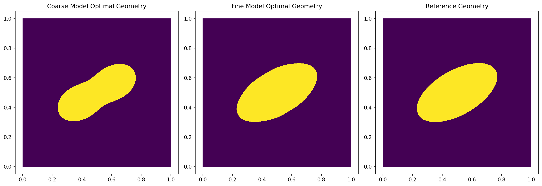
Note
The left image shows the optimized geometry with the coarse model, the middle image shows the optimized geometry with the fine model (with the space mapping technique), and the right image shows the reference geometry, which we were trying to reconstruct. We can see that using the coarse model alone as approximation of the original problem does not work sufficiently well as we recover some kind of rotated peanut shape, instead of a rotated ellipse. However, we see that the space mapping approach works very well for recovering the desired ellipse.