Treatment of additional constraints#
Problem Formulation#
In this demo we investigate cashocs for solving PDE constrained optimization problems with additional constraints. To do so, we investigate the “mother problem” of PDE constrained optimization, i.e.,
Here, we have four additional constraints, each for one quarter of the unit square \(\Omega = (0,1)^2\), indicated by \((b,l)\) for bottom left, \((b,r)\) for bottom right, \((t,l)\) for top left, and \((t,r)\) for top right.
In the following, we will describe how to solve this problem using cashocs.
Implementation#
The complete python code can be found in the file demo_constraints.py and the
corresponding config can be found in config.ini.
Initialization#
The beginning of the program is nearly the same as for Distributed Control of a Poisson Problem
from fenics import *

import cashocs

cashocs.set_log_level(cashocs.log.INFO)
config = cashocs.load_config("config.ini")
mesh, subdomains, boundaries, dx, ds, dS = cashocs.regular_mesh(32)
V = FunctionSpace(mesh, "CG", 1)

y = Function(V)
p = Function(V)
u = Function(V)

e = inner(grad(y), grad(p)) * dx - u * p * dx

bcs = cashocs.create_dirichlet_bcs(V, Constant(0), boundaries, [1, 2, 3, 4])

y_d = Expression("sin(2*pi*x[0])*sin(2*pi*x[1])", degree=1)
alpha = 1e-4
J = cashocs.IntegralFunctional(
    Constant(0.5) * (y - y_d) * (y - y_d) * dx + Constant(0.5 * alpha) * u * u * dx
)
Definition of the additional constraints#
In the following, we define the additional constraints we want to consider together with the PDE constraint. In this case, we only have state constraints, but additional constraints on the control variables can be treated completely analogously.
First, we define the four quarters of the unit square
bottom_left = Expression("(x[0] <= 0.5) && (x[1] <= 0.5) ? 1.0 : 0.0", degree=0)
bottom_right = Expression("(x[0] >= 0.5) && (x[1] <= 0.5) ? 1.0 : 0.0", degree=0)
top_left = Expression("(x[0] <= 0.5) && (x[1] >= 0.5) ? 1.0 : 0.0", degree=0)
top_right = Expression("(x[0] >= 0.5) && (x[1] >= 0.5) ? 1.0 : 0.0", degree=0)
The four Expressions above are indicator functions for the respective quarters, which allows us to implement the constraints easily.
Next, we define the pointwise equality constraint we have on the lower left quarter.
To do so, we use cashocs.EqualityConstraint as follows
pointwise_equality_constraint = cashocs.EqualityConstraint(
    bottom_left * y, 0.0, measure=dx
)
Here, the first argument is the left-hand side of the equality constraint, namely the
indicator function for the lower left quarter multiplied by the state variable y.
The next argument is the right-hand side of the equality constraint, i.e.,
\(c_{b,l}\) which we choose as 0 in this example. Finally, the keyword argument
measure is used to specify the integration measure that should be used to
define where the constraint is given. Typical examples are a volume measure (dx, as
it is the case here) or surface measure (ds, which could be used if we wanted to
pose the constraint only on the boundary).
Let’s move on to the next constraint. Again, we have an equality constraint, but now it is a scalar value which is constrained, and its given by the integral over some integrand. This is the general form in which cashocs can deal with such scalar constraints. Let’s see how we can define this constraint in cashocs
integral_equality_constraint = cashocs.EqualityConstraint(
    bottom_right * pow(y, 2) * dx, 0.01
)
Here, we again use the cashocs.EqualityConstraint class, as before. The
difference is that now, the first argument is the UFL form of the integrand, in this
case \(y^2\) multiplied by the indicator function of the bottom right quarter, i.e.,
the left-hand side of the constraint. The second and final argument for this
constraint is right-hand side of the constraint, i.e., \(c_{b,r}\), which we choose as
0.01 in this example.
Let’s move on to the interesting case of inequality constraints. Let us first consider
a setting similar to before, where the constraint’s left-hand side is given by an
integral over some integrand. We define this integral inequality constraint via the
cashocs.InequalityConstraint class
integral_inequality_constraint = cashocs.InequalityConstraint(
    top_left * y * dx, lower_bound=-0.025
)
Here, as before, the first argument is the left-hand side of the constraint, i.e., the
UFL form of the integrand, in this case \(y\) times the indicator function of the top
left quarter, which is to be integrated over the measure dx. The second
argument lower_bound = -0.025 specifies the lower bound for this inequality
constraint, that means, that \(c_{t,l} = -0.025\) in our case.
Finally, let us take a look at the case of pointwise inequality constraint. This is,
as before, implemented via the cashocs.InequalityConstraint class
pointwise_inequality_constraint = cashocs.InequalityConstraint(
    top_right * y, upper_bound=0.25, measure=dx
)
Here, again the first argument is the function on the left-hand side of the
constraint, i.e., \(y\) times the indicator function of the top right quarter. The
second argument, upper_bound=0.25, defines the right-hand side of the
constraint, i.e., we choose \(c_{t,r} = 0.25\). Finally, as for the pointwise equality
constraint, we specify the integration measure for which the constraint is posed, in
our case measure=dx, as we consider the constraint pointwise in the domain
\(\Omega\).
Note
For bilateral inequality constraints we can use both keyword arguments
upper_bound and lower_bound to define both bounds for the
constraint.
As is usual in cashocs, once we have defined multiple constraints, we gather them into a list to pass them to the optimization routines
constraints = [
    pointwise_equality_constraint,
    integral_equality_constraint,
    integral_inequality_constraint,
    pointwise_inequality_constraint,
]
Finally, we define the optimization problem. As we deal with additional constraints,
we do not use a cashocs.OptimalControlProblem, but use a
cashocs.ConstrainedOptimalControlProblem, which can be used to deal with
these additional constaints. As usual, we can solve the problem with its
solve method
problem = cashocs.ConstrainedOptimalControlProblem(
    e, bcs, J, y, u, p, constraints, config
)
problem.solve(method="AL")
Note
To be able to treat (nearly) arbitrary types of constraints, cashocs regularizes
these using either an augmented Lagrangian method or a quadratic penalty method.
Which method is used can be specified via the keyword argument method, which
is chosen to be an augmented Lagrangian method ('AL') in this demo.
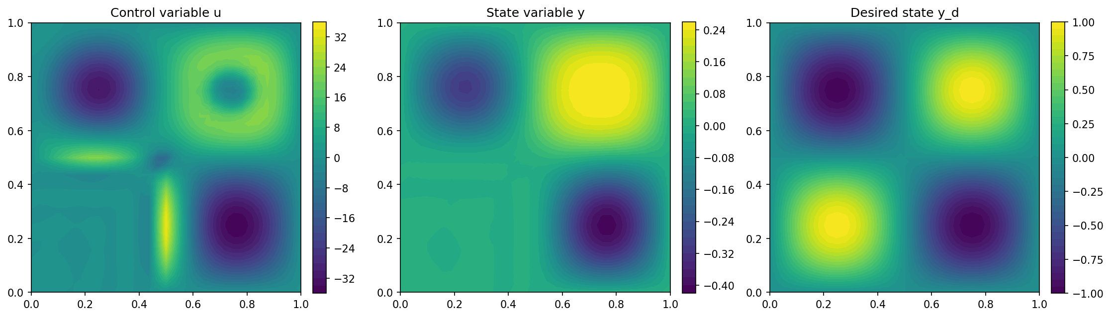
Finally, we visualize the result with the following code
import matplotlib.pyplot as plt

plt.figure(figsize=(15, 5))

plt.subplot(1, 3, 1)
fig = plot(u)
plt.colorbar(fig, fraction=0.046, pad=0.04)
plt.title("Control variable u")

plt.subplot(1, 3, 2)
fig = plot(y)
plt.colorbar(fig, fraction=0.046, pad=0.04)
plt.title("State variable y")

plt.subplot(1, 3, 3)
fig = plot(y_d, mesh=mesh)
plt.colorbar(fig, fraction=0.046, pad=0.04)
plt.title("Desired state y_d")

plt.tight_layout()
# plt.savefig("./img_constraints.png", dpi=150, bbox_inches="tight")
and the result should look like this