Boundary conditions for control variables

Problem Formulation

In this demo we investigate cashocs for solving PDE constrained optimization problems with additional boundary conditions for the control variables. Our problem is given by

\[\begin{split} \begin{align} &\min\; J(y,u) = \frac{1}{2} \int_{\Omega} \left( y - y_d \right)^2 \text{ d}x + \frac{\alpha}{2} \int_{\Omega} u^2 \text{ d}x \\ &\text{ subject to } \qquad \begin{alignedat}[t]{2} -\Delta y &= u \quad &&\text{ in } \Omega,\\ y &= 0 \quad &&\text{ on } \Gamma, \\ u &= u_{\Gamma} \quad &&\text{ on } \Gamma, \end{alignedat} \end{align} \end{split}\]

Here, we consider the control variable \(u\) in \(H^1_\Gamma(\Omega) = \{ v \in H^1(\Omega) \vert v = u_\Gamma \text{ on } \Gamma \}\).

In the following, we will describe how to solve this problem using cashocs.

Implementation

The complete python code can be found in the file demo_constraints.py and the corresponding config can be found in config.ini.

Initialization

The beginning of the program is nearly the same as for Distributed Control of a Poisson Problem

from fenics import *

import cashocs

cashocs.set_log_level(cashocs.LogLevel.INFO)
config = cashocs.load_config("config.ini")
mesh, subdomains, boundaries, dx, ds, dS = cashocs.regular_mesh(25)
V = FunctionSpace(mesh, "CG", 1)

y = Function(V)
p = Function(V)
u = Function(V)

e = inner(grad(y), grad(p)) * dx - u * p * dx

bcs = cashocs.create_dirichlet_bcs(V, Constant(0), boundaries, [1, 2, 3, 4])

y_d = Expression("sin(2*pi*x[0])*sin(2*pi*x[1])", degree=1)
alpha = 1e-6
J = cashocs.IntegralFunctional(
    Constant(0.5) * (y - y_d) * (y - y_d) * dx + Constant(0.5 * alpha) * u * u * dx
)

Scalar product and boundary conditions for the control variable

Now, we can first define the scalar product for the control variable \(u\), which we choose as the standard \(H^1_0(\Omega)\) scalar product. This can be implemented as follows in cashocs

scalar_product = dot(grad(TrialFunction(V)), grad(TestFunction(V))) * dx

Moreover, we define the list of boundary conditions for the control variable as usual in FEniCS and cashocs with the help of cashocs.create_dirichlet_bcs()

control_bcs = cashocs.create_dirichlet_bcs(V, Constant(100.0), boundaries, [1, 2, 3, 4])

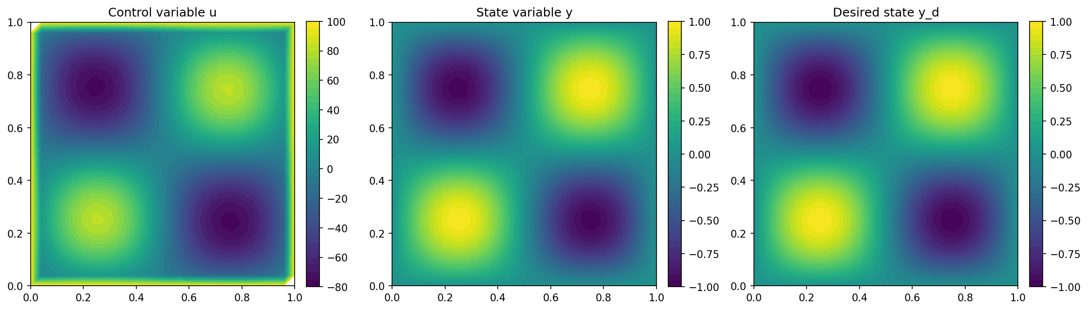
Here, we have chosen a value of \(u_\Gamma = 100\) for this particular demo, in order to be able to visually see, whether the proposed method works.

Finally, we can set up and solve the optimization problem as usual

ocp = cashocs.OptimalControlProblem(
    e,
    bcs,
    J,
    y,
    u,
    p,
    config=config,
    riesz_scalar_products=scalar_product,
    control_bcs_list=control_bcs,
)
ocp.solve()

where the only additional parts in comparison to Distributed Control of a Poisson Problem are the keyword arguments riesz_scalar_products, which was already covered in Neumann Boundary Control, and control_bcs_list, which we have defined previously.

After solving this problem with cashocs, we visualize the solution with the code

import matplotlib.pyplot as plt

plt.figure(figsize=(15, 5))

plt.subplot(1, 3, 1)
fig = plot(u)
plt.colorbar(fig, fraction=0.046, pad=0.04)
plt.title("Control variable u")

plt.subplot(1, 3, 2)
fig = plot(y)
plt.colorbar(fig, fraction=0.046, pad=0.04)
plt.title("State variable y")

plt.subplot(1, 3, 3)
fig = plot(y_d, mesh=mesh)
plt.colorbar(fig, fraction=0.046, pad=0.04)
plt.title("Desired state y_d")

plt.tight_layout()
# plt.savefig("./img_control_boundary_conditions.png", dpi=150, bbox_inches="tight")

and the result should look like this