Dirichlet Boundary Control

Problem Formulation

In this demo, we investigate how Dirichlet boundary control is possible with cashocs. To do this, we have to employ the so-called Nitsche method, which we briefly recall in the following. Our model problem for this example is given by

\[\begin{split} \begin{align} &\min\; J(y,u) = \frac{1}{2} \int_{\Omega} \left( y - y_d \right)^2 \text{ d}x + \frac{\alpha}{2} \int_{\Gamma} u^2 \text{ d}s \\ &\text{ subject to } \qquad \begin{alignedat}[t]{2} -\Delta y &= 0 \quad &&\text{ in } \Omega,\\ y &= u \quad &&\text{ on } \Gamma. \end{alignedat} \end{align} \end{split}\]

In contrast to our previous problems, the control now enters the problem via a Dirichlet boundary condition. However, we cannot apply these via a fenics.DirichletBC, because for cashocs to work properly, the controls, states, and adjoints are only allowed to appear in UFL forms. Nitsche’s Method circumvents this problem by imposing the boundary conditions in the weak form directly. Let us first briefly recall this method.

Nitsche’s Method

Consider the Laplace problem

\[\begin{split} \begin{alignedat}{2} -\Delta y &= 0 \quad &&\text{ in } \Omega,\\ y &= u \quad &&\text{ on } \Gamma. \end{alignedat} \end{split}\]

We can derive a weak form for this equation in \(H^1(\Omega)\) (not \(H^1_0(\Omega)\)) by multiplying the equation by a test function \(p \in H^1(\Omega)\) and applying the divergence theorem

\[ \int_\Omega - \Delta y p \text{ d}x = \int_\Omega \nabla y \cdot \nabla p \text{ d}x - \int_\Gamma (\nabla y \cdot n) p \text{ d}s. \]

This weak form is the starting point for Nitsche’s method. First of all, observe that this weak form is not symmetric anymore. To restore symmetry of the problem, we can use the Dirichlet boundary condition and “add a zero” by adding \(\int_\Gamma \nabla p \cdot n (y - u) \text{ d}s\). This gives the weak form

\[ \int_\Omega \nabla y \cdot \nabla p \text{ d}x - \int_\Gamma (\nabla y \cdot n) p \text{ d}s - \int_\Gamma (\nabla p \cdot n) y \text{ d}s = \int_\Gamma (\nabla p \cdot n) u \text{ d}s. \]

However, one can show that this weak form is not coercive. Hence, Nitsche’s method adds another zero to this weak form, namely \(\int_\Gamma \eta (y - u) p \text{ d}s\), which yields the coercivity of the problem if \(\eta\) is sufficiently large. Hence, we consider the following weak form

\[ \int_\Omega \nabla y \cdot \nabla p \text{ d}x - \int_\Gamma (\nabla y \cdot n) p \text{ d}s - \int_\Gamma (\nabla p \cdot n) y \text{ d}s + \eta \int_\Gamma y p \text{ d}s = \int_\Gamma (\nabla p \cdot n) u \text{ d}s + \eta \int_\Gamma u p \text{ d}s, \]

and this is the form we implement for this problem.

For a detailed introduction to Nitsche’s method, we refer to Assous and Michaeli - A numerical method for handling boundary and transmission conditions in some linear partial differential equations.

Note

To ensure convergence of the method when the mesh is refined, the parameter \(\eta\) is scaled in dependence with the mesh size. In particular, we use a scaling of the form

\[ \eta = \frac{\bar{\eta}}{h}, \]

where \(h\) is the diameter of the current mesh element.

Implementation

The complete python code can be found in the file demo_dirichlet_control.py and the corresponding config can be found in config.ini.

Initialization

The beginning of the program is nearly the same as for Distributed Control of a Poisson Problem

from fenics import *
import numpy as np

import cashocs

config = cashocs.load_config("config.ini")
mesh, subdomains, boundaries, dx, ds, dS = cashocs.regular_mesh(50)
n = FacetNormal(mesh)
h = MaxCellEdgeLength(mesh)
V = FunctionSpace(mesh, "CG", 1)

y = Function(V)
p = Function(V)
u = Function(V)

The only difference is, that we now also define n, which is the outer unit normal vector on \(\Gamma\), and h, which is the maximum length of an edge of the respective finite element (during assemly).

Then, we define the Dirichlet boundary conditions, which are enforced strongly. As we use Nitsche’s method to implement the boundary conditions on the entire boundary, there are no strongly enforced ones left, and we define

bcs = []

Hint

Alternatively, we could have also written

bcs = None

which yields exactly the same result, i.e., no strongly enforced Dirichlet boundary conditions.

Definition of the PDE and optimization problem via Nitsche’s method

We implement the weak form using Nitsche’s method, as described above, which is given by the code segment

eta = Constant(1e4)
e = (
    inner(grad(y), grad(p)) * dx
    - inner(grad(y), n) * p * ds
    - inner(grad(p), n) * (y - u) * ds
    + eta / h * (y - u) * p * ds
    - Constant(1) * p * dx
)

Finally, we can define the cost functional similarly to Neumann Boundary Control

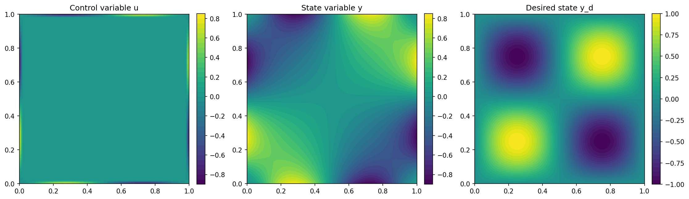
y_d = Expression("sin(2*pi*x[0])*sin(2*pi*x[1])", degree=1)
alpha = 1e-4
J = cashocs.IntegralFunctional(
    Constant(0.5) * (y - y_d) * (y - y_d) * dx + Constant(0.5 * alpha) * u * u * ds
)

As in Neumann Boundary Control, we have to define a scalar product on \(L^2(\Gamma)\) to get meaningful results (as the control is only defined on the boundary), which we do with

scalar_product = TrialFunction(V) * TestFunction(V) * ds

Solution of the optimization problem

The optimal control problem is solved with the usual syntax

ocp = cashocs.OptimalControlProblem(
    e, bcs, J, y, u, p, config=config, riesz_scalar_products=scalar_product
)
ocp.solve()

In the end, we validate whether the boundary conditions are applied correctly using this approach. Therefore, we first compute the indices of all DOF’s that lie on the boundary via

bcs = cashocs.create_dirichlet_bcs(V, 1, boundaries, [1, 2, 3, 4])
bdry_idx = Function(V)
[bc.apply(bdry_idx.vector()) for bc in bcs]
mask = np.where(bdry_idx.vector()[:] == 1)[0]

Then, we restrict both y and u to the boundary by

y_bdry = Function(V)
u_bdry = Function(V)
y_bdry.vector()[mask] = y.vector()[mask]
u_bdry.vector()[mask] = u.vector()[mask]

Finally, we compute the relative errors in the \(L^\infty(\Gamma)\) and \(L^2(\Gamma)\) norms and print the result

error_inf = (
    np.max(np.abs(y_bdry.vector()[:] - u_bdry.vector()[:]))
    / np.max(np.abs(u_bdry.vector()[:]))
    * 100
)
error_l2 = (
    np.sqrt(assemble((y - u) * (y - u) * ds)) / np.sqrt(assemble(u * u * ds)) * 100
)
print("Error regarding the (weak) imposition of the boundary values")
print("Error L^\infty: " + format(error_inf, ".3e") + " %")
print("Error L^2: " + format(error_l2, ".3e") + " %")

We see, that with eta = 1e4 we get a relative error of under 5e-3 % in the \(L^\infty(\Omega)\) norm, and under 5e-4 in the \(L^2(\Omega)\) norm, which is sufficient for applications.

Finally, we visualize our results with the code

import matplotlib.pyplot as plt

plt.figure(figsize=(15, 5))

plt.subplot(1, 3, 1)
fig = plot(u)
plt.colorbar(fig, fraction=0.046, pad=0.04)
plt.title("Control variable u")

plt.subplot(1, 3, 2)
fig = plot(y)
plt.colorbar(fig, fraction=0.046, pad=0.04)
plt.title("State variable y")

plt.subplot(1, 3, 3)
fig = plot(y_d, mesh=mesh)
plt.colorbar(fig, fraction=0.046, pad=0.04)
plt.title("Desired state y_d")

plt.tight_layout()
# plt.savefig('./img_dirichlet_control.png', dpi=150, bbox_inches='tight')

and the resulting output should look like