Distributed Control of a Stokes Problem#
Problem Formulation#
In this demo we investigate how cashocs can be used to treat a different kind of PDE constraint, in particular, we investigate a Stokes problem. The optimization problem reads as follows
In contrast to the other demos, here we denote by \(u\) the velocity of a fluid and by \(p\) its pressure, which are the two state variables. The control is now denoted by \(c\) and acts as a volume source for the system. The tracking type cost functional again aims at getting the velocity u close to some desired velocity \(u_d\).
For this example, the geometry is again given by \(\Omega = (0,1)^2\), and we take a look at the setting of the well known lid driven cavity benchmark here. In particular, the boundary conditions are classical no slip boundary conditions at the left, right, and bottom sides of the square. On the top (or the lid), a velocity \(u_\text{dir}\) is prescribed, pointing into the positive x-direction. Note, that since this problem has Dirichlet conditions on the entire boundary, the pressure is only determined up to a constant, and hence we have to specify another condition to ensure uniqueness. For this demo we choose another Dirichlet condition, specifying the value of the pressure at a single point in the domain. Alternatively, we could have also required that, e.g., the integral of the velocity \(u\) over \(\Omega\) vanishes (the implementation would then only be slightly longer, but not as intuitive). An example of how to treat such an additional constraint in FEniCS and cashocs can be found in Inverse Problem in Electric Impedance Tomography.
Implementation#
The complete python code can be found in the file demo_stokes.py,
and the corresponding config can be found in config.ini.
Initialization#
The initialization is the same as in Distributed Control of a Poisson Problem, i.e.,
from fenics import *

import cashocs

config = cashocs.load_config("./config.ini")
mesh, subdomains, boundaries, dx, ds, dS = cashocs.regular_mesh(30)
For the solution of the Stokes (and adjoint Stokes) system, which have a saddle point structure, we have to choose LBB stable elements or a suitable stabilization, see e.g. Ern and Guermond - Theory and Practice of Finite Elements. For this demo, we use the classical Taylor-Hood elements of piecewise quadratic Lagrange elements for the velocity, and piecewise linear ones for the pressure, which are LBB-stable. These are defined as
v_elem = VectorElement("CG", mesh.ufl_cell(), 2)
p_elem = FiniteElement("CG", mesh.ufl_cell(), 1)
V = FunctionSpace(mesh, MixedElement([v_elem, p_elem]))
U = VectorFunctionSpace(mesh, "CG", 1)
Moreover, we have defined the control space U as
fenics.FunctionSpace with piecewise linear Lagrange elements.
Next, we set up the corresponding function objects, as follows
up = Function(V)
u, p = split(up)
vq = Function(V)
v, q = split(vq)
c = Function(U)
Here, up plays the role of the state variable, having components u
and p, which are extracted using the ufl.split() command. The
adjoint state vq is structured in exactly the same fashion. See
Coupled Problems - Monolithic Approach for more details. Similarly to there, v will
play the role of the adjoint velocity, and q the one of the adjoint
pressure.
Next up is the definition of the Stokes system. This can be done via
e = inner(grad(u), grad(v)) * dx - p * div(v) * dx - q * div(u) * dx - inner(c, v) * dx
Note
Note, that we have chosen to consider the incompressibility condition with a negative sign. This is used to make sure that the resulting system is symmetric (but indefinite) which can simplify its solution. Using the positive sign for the divergence constraint would instead lead to a non-symmetric but positive-definite system.
The boundary conditions for this system can be defined as follows
def pressure_point(x, on_boundary):
    return near(x[0], 0) and near(x[1], 0)
no_slip_bcs = cashocs.create_dirichlet_bcs(
    V.sub(0), Constant((0, 0)), boundaries, [1, 2, 3]
)
lid_velocity = Expression(("4*x[0]*(1-x[0])", "0.0"), degree=2)
bc_lid = DirichletBC(V.sub(0), lid_velocity, boundaries, 4)
bc_pressure = DirichletBC(V.sub(1), Constant(0), pressure_point, method="pointwise")
bcs = no_slip_bcs + [bc_lid, bc_pressure]
Here, we first define the point \(x^\text{pres}\), where the pressure is set to 0.
Afterwards, we use the cashocs function create_dirichlet_bcs to quickly create the no slip conditions at the left,
right, and bottom of the cavity. Next, we define the Dirichlet velocity \(u_\text{dir}\)
for the lid of the cavity as a fenics.Expression, and create a
corresponding boundary condition. Finally, the Dirichlet condition for the pressure is
defined. Note that in order to make this work, one has to specify the keyword argument
method='pointwise'.
Defintion of the optimization problem#
The definition of the optimization problem is in complete analogy to the previous
ones we considered. The only difference is the fact that we now have to use
ufl.inner() to multiply the vector valued functions u,
u_d and c.
alpha = 1e-5
u_d = Expression(
    (
        "sqrt(pow(x[0], 2) + pow(x[1], 2))*cos(2*pi*x[1])",
        "-sqrt(pow(x[0], 2) + pow(x[1], 2))*sin(2*pi*x[0])",
    ),
    degree=2,
)
J = cashocs.IntegralFunctional(
    Constant(0.5) * inner(u - u_d, u - u_d) * dx
    + Constant(0.5 * alpha) * inner(c, c) * dx
)
As in Coupled Problems - Monolithic Approach, we then set up the optimization problem
ocp and solve it with the command
ocp.solve()
ocp = cashocs.OptimalControlProblem(e, bcs, J, up, c, vq, config=config)
ocp.solve()
For post-processing, we then create deep copies of the single components of the state and the adjoint variables with
u, p = up.split(True)
and we then visualize the results with
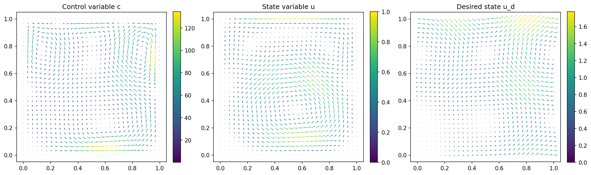
import matplotlib.pyplot as plt

plt.figure(figsize=(15, 5))

plt.subplot(1, 3, 1)
fig = plot(c)
plt.colorbar(fig, fraction=0.046, pad=0.04)
plt.title("Control variable c")

plt.subplot(1, 3, 2)
fig = plot(u)
plt.colorbar(fig, fraction=0.046, pad=0.04)
plt.title("State variable u")

plt.subplot(1, 3, 3)
fig = plot(u_d, mesh=mesh)
plt.colorbar(fig, fraction=0.046, pad=0.04)
plt.title("Desired state u_d")

plt.tight_layout()
# plt.savefig('./img_stokes.png', dpi=150, bbox_inches='tight')
so that the results look like this