Distributed Control of a Poisson Problem#
Problem Formulation#
In this demo we investigate the basics of cashocs for optimal control problems. To do so, we investigate the “mother problem” of PDE constrained optimization, i.e.,
(see, e.g., Tröltzsch - Optimal Control of Partial Differential Equations or Hinze, Pinnau, Ulbrich, and Ulbrich - Optimization with PDE constraints.
For this first example, we do not consider control constraints, but search for an optimal control u in the entire space \(L^2(\Omega)\), for the sake of simplicitiy. For the domain under consideration, we use the unit square \(\Omega = (0, 1)^2\), since this is built into cashocs.
In the following, we will describe how to solve this problem using cashocs. Moreover, we also detail alternative / equivalent FEniCS code which could be used to define the problem instead.
Implementation#
The complete python code can be found in the file
demo_poisson.py
and the corresponding config can be found in
config.ini.
Initialization#
We begin by importing FEniCS and cashocs. For the sake of better readability we use a wildcard import for FEniCS
from fenics import *

import cashocs
Afterwards, we can specify the so-called log level of cashocs. This is done in the line
cashocs.log.set_log_level(cashocs.log.INFO)
Hint
There are a total of five levels of verbosity, given by
cashocs.log.DEBUG, cashocs.log.INFO,
cashocs.log.WARNING, cashocs.log.ERROR,
and cashocs.log.CRITICAL. The default value is INFO, which
would also be selected if the cashocs.log.set_log_level() method would not
have been called.
Next, we have to load the config file which loads the user’s input parameters into the script. For a detailed documentation of the config files and the parameters within, we refer to Documentation of the Config Files for Optimal Control Problems. The config is then loaded via
config = cashocs.load_config("config.ini")
Next up, we have to define the state equation. This mostly works with usual FEniCS syntax. In cashocs, we can quickly generate meshes for squares and cubes, as well as import meshes generated by Gmsh, for more complex geometries. In this example we take a built-in unit square as example. This is generated via
mesh, subdomains, boundaries, dx, ds, dS = cashocs.regular_mesh(25)
The input for regular_mesh determines the number of elements that
are placed along each axis of the square. Note, that the mesh could be
further manipulated with additional, optional arguments, and we
refer to regular_mesh for more infos. Note,
that the subdomains object is a (empty) MeshFunction, and that
boundaries is a MeshFunction that contains markers for the following
boundaries
The left side of the square is marked by 1
The right side is marked by 2
The bottom is marked by 3
The top is marked by 4,
as defined in regular_mesh.
With the geometry defined, we create a function space with the classical FEniCS syntax
V = FunctionSpace(mesh, "CG", 1)
which creates a function space of continuous, linear Lagrange elements.
Definition of the state equation#
To describe the state system in cashocs, we use (almost) standard
FEniCS syntax, and the differences will be highlighted in the
following. First, we define a fenics.Function y that models our
state variable \(y\), and a fenics.Function p that models
the corresponding adjoint variable \(p\) via
y = Function(V)
p = Function(V)
Next up, we analogously define the control variable as fenics.Function
u
u = Function(V)
This enables us to define the weak form of the state equation,
which is tested not with a fenics.TestFunction but with the adjoint
variable p via the classical FEniCS / UFL syntax
e = inner(grad(y), grad(p)) * dx - u * p * dx
Note
For the clasical definition of this weak form with FEniCS one would write the following code
y = TrialFunction(V)
p = TestFunction(V)
u = Function(V)
a = inner(grad(y), grad(p)) * dx
L = u * p * dx
as this is a linear problem. However, to have greater flexibility we have to treat the problems as being potentially nonlinear. In this case, the classical FEniCS formulation for this as nonlinear problem would be
y = Function(V)
p = TestFunction(V)
u = Function(V)
F = inner(grad(y), grad(p)) * dx -u * p * dx
which could then be solved via the fenics.solve() interface. This
formulation, which comes more naturally for nonlinear
variational problems (see the
FEniCS examples)
is closer to the one in cashocs. However, for the use with cashocs, the state variable
\(y\) must not be a fenics.TrialFunction, and the adjoint variable
\(p\) must not be a fenics.TestFunction. They have to be
defined as regular fenics.Function objects, otherwise the code will not
work properly.
After defining the weak form of the state equation, we now specify the corresponding (homogeneous) Dirichlet boundary conditions via
bcs = cashocs.create_dirichlet_bcs(V, Constant(0), boundaries, [1, 2, 3, 4])
This creates Dirichlet boundary conditions with value 0 at the boundaries 1,2,3, and 4, i.e., everywhere.
Hint
Classically, these boundary conditions could also be defined via
def boundary(x, on_bdry):
    return on_boundary
bc = DirichletBC(V, Constant(0), boundary)
which would yield a single DirichletBC object, instead of the list returned by
create_dirichlet_bcs. Any of the many
methods for defining the boundary conditions works here, as long as it is valid input
for the fenics.solve() function.
With the above description, we see that defining the state system
for cashocs is nearly identical to defining it with FEniCS,
the only major difference lies in the definition of the state
and adjoint variables as fenics.Function objects, instead of
fenics.TrialFunction and fenics.TestFunction.
Definition of the cost functional#
Now, we have to define the optimal control problem which we do
by first specifying the cost functional. To do so, we define the
desired state \(y_d\) as an fenics.Expression y_d, i.e.,
y_d = Expression("sin(2*pi*x[0])*sin(2*pi*x[1])", degree=1)
Alternatively, y_d could also be a fenics.Function or any other
object that is usable in an UFL form (e.g. generated with
fenics.SpatialCoordinate()).
Then, we define the regularization parameter \(\alpha\) and the tracking-type cost functional via the commands
alpha = 1e-6
J = cashocs.IntegralFunctional(
    Constant(0.5) * (y - y_d) * (y - y_d) * dx + Constant(0.5 * alpha) * u * u * dx
)
The cost functional is defined via the cashocs.IntegralFunctional, which
means that we only have to define the cost functional’s integrand, which will then
further be treated by cashocs as needed for the optimization. These definitions are
also classical in the sense that they would have to be performed in this (or a
similar) way in FEniCS when one would want to evaluate the (reduced) cost functional,
so that we have only very little overhead.
Definition of the optimization problem and its solution#
Finally, we set up an
OptimalControlProblem ocp and
then directly solve it with the method ocp.solve()
ocp = cashocs.OptimalControlProblem(e, bcs, J, y, u, p, config=config)
ocp.solve()
Hint
Note that the solve command without
any additional keyword arguments leads to cashocs using the settings defined in the
config file. However, there are some options that can be directly set with keyword
arguments for the solve call. These
are
algorithm: Specifies which solution algorithm shall be used.rtol: The relative tolerance for the optimization algorithm.atol: The absolute tolerance for the optimization algorithm.max_iter: The maximum amount of iterations that can be carried out.
Hence, we could also use the command
ocp.solve('lbfgs', 1e-3, 0.0, 100)
to solve the optimization problem with the L-BFGS method, a relative tolerance of
1e-3, no absolute tolerance, and a maximum of 100 iterations.
The possible values for these arguments are the same as the corresponding ones in the config file. This just allows for some shortcuts, e.g., when one wants to quickly use a different solver.
Note, that it is not strictly necessary to supply config files in cashocs. In this
case, the user has to follow the above example and specify at least the solution
algorithm via the solve method.
However, it is very strongly recommended to use config files with cashocs as
they allow a detailed tuning of its behavior.
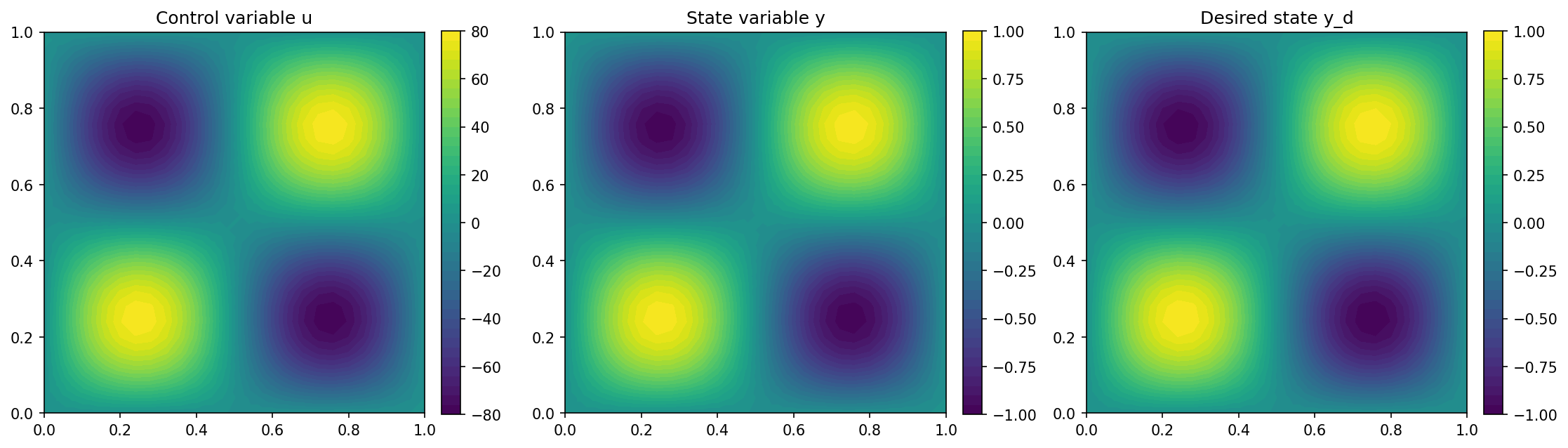
Finally, we visualize the results using matplotlib and the following code ::
import matplotlib.pyplot as plt

plt.figure(figsize=(15, 5))

plt.subplot(1, 3, 1)
fig = plot(u)
plt.colorbar(fig, fraction=0.046, pad=0.04)
plt.title("Control variable u")

plt.subplot(1, 3, 2)
fig = plot(y)
plt.colorbar(fig, fraction=0.046, pad=0.04)
plt.title("State variable y")

plt.subplot(1, 3, 3)
fig = plot(y_d, mesh=mesh)
plt.colorbar(fig, fraction=0.046, pad=0.04)
plt.title("Desired state y_d")

plt.tight_layout()
# plt.savefig('./img_poisson.png', dpi=150, bbox_inches='tight')
The output should look like this