Writing and Reading XDMF Files#

cashocs can be used to store XDMF files of the current states, adjoints, and gradients. This has great use for visualization and post-processing. The output of these files is usually controlled via the configuration file, see the corresponding documentation for optimal control and shape optimization.

In this tutorial, we show how cashocs can be used to store these files, but also how these files can be used to read the solutions into python again, so that a post-processing can also occur inside python, not only with paraview. To do so, we consider the same problem as in Shape Optimization with a Poisson Problem, which we do not again recall here.

Implementation#

The complete python code can be found in the file demo_xdmf_io.py, and the corresponding config can be found in config.ini.

Automatically writing XDMF files#

Let us start our discussion with solving the shape optimization problem, where we use code in complete analogy to Shape Optimization with a Poisson Problem. The only difference lies in the config file, where we use the following

config.ini#

[Output]
save_state = True
save_adjoint = True
save_gradient = True

This means, that when we now use cashocs to solve the problem, the output is stored to a directory, which is specified in the result_dir of the Output Section of the config file. As we have not specified a directory, the files will be created in the default location ./results, and the XDMF files will be stored in ./results/checkpoints.

The code for solving the problem is as follows

from fenics import *

import matplotlib.pyplot as plt

import cashocs

config = cashocs.load_config("./config.ini")
mesh, subdomains, boundaries, dx, ds, dS = cashocs.import_mesh("./mesh/mesh.xdmf")

V = FunctionSpace(mesh, "CG", 1)
u = Function(V)
p = Function(V)

x = SpatialCoordinate(mesh)
f = 2.5 * pow(x[0] + 0.4 - pow(x[1], 2), 2) + pow(x[0], 2) + pow(x[1], 2) - 1

e = inner(grad(u), grad(p)) * dx - f * p * dx
bcs = DirichletBC(V, Constant(0), boundaries, 1)

J = cashocs.IntegralFunctional(u * dx)

sop = cashocs.ShapeOptimizationProblem(e, bcs, J, u, p, boundaries, config=config)
sop.solve()

After we have run this code, we can see that now a directory ./results exists and that the XDMF files are located in ./results/checkpoints, as expected.

Reading the XDMF files back into python#

To read the stored functions back into python, we can make use of the function cashocs.io.read_function_from_xdmf(), which works as follows

u_init = cashocs.io.read_function_from_xdmf(
    "./results/checkpoints/state_0.xdmf", "state_0", "CG", 1, step=0
)

The function works as follows. In the first argument, we have to specify the location of the file which we want to read. The second argument is the name of the function. Cashocs names these functions depending on whether they are a state, adjoint, or control variable or whether they are gradient-type functions. State variables are named 'state_i' where i denotes the index of the state variable, in case multiple ones are used. The same is true for adjoint variables, control variables, and gradients, where the names are 'adjoint_i', 'control_i', and 'gradient_i' or 'shape_gradient_i'.

Hint

One can easily deduce the name of a variable stored in an XDMF file written by cashocs. If the file is named 'name_i.xdmf', the name of the function is 'name_i'. For example, when using multiple variables or problems with mixed spaces, the outputs could, e.g., have the names 'state_1_2.xdmf', so that the corresponding name would be 'state_1_sub_2'

Warning

The only exception to the above rule are shape gradients. There, the files are called 'shape_gradient.xdmf', but the name of the functions is analogous to the one for optimal control, i.e., it is always 'gradient_0'.

The third parameter for cashocs.io.read_function_from_xdmf() is the name of the finite element space, which was used when initially creating the function space for the function. As we used linear Lagrange elements, we have to use 'CG' here. The fourth argument specifies the degree of the finite element, which is 1 in this case. Finally, the keyword argument step is used to indicate at which iteration we would like to read the function. For this example we have chosen step=0, so that we read the state variable at the initial iteration.

Let us now also read the state variable at the last iteration, which we do with the line

u_final = cashocs.io.read_function_from_xdmf(
    "./results/checkpoints/state_0.xdmf", "state_0", "CG", 1, step=11
)

Let us now compare these functions in python, with the help of matplotlib.

plt.figure(figsize=(10, 10))
plt.subplot(1, 2, 1)
plot(u_init)
plt.title("State variable at initial iteration")

plt.subplot(1, 2, 2)
plot(u_final)
plt.title("State variable at final iteration")

plt.tight_layout()
# plt.savefig("./img_states.png", dpi=150, bbox_inches="tight")

The result looks as follows

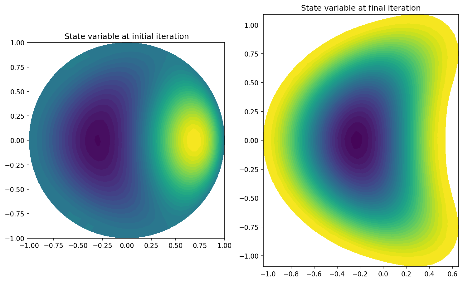
Here, we can nicely see that we indeed have loaded variables from totally different iterations.

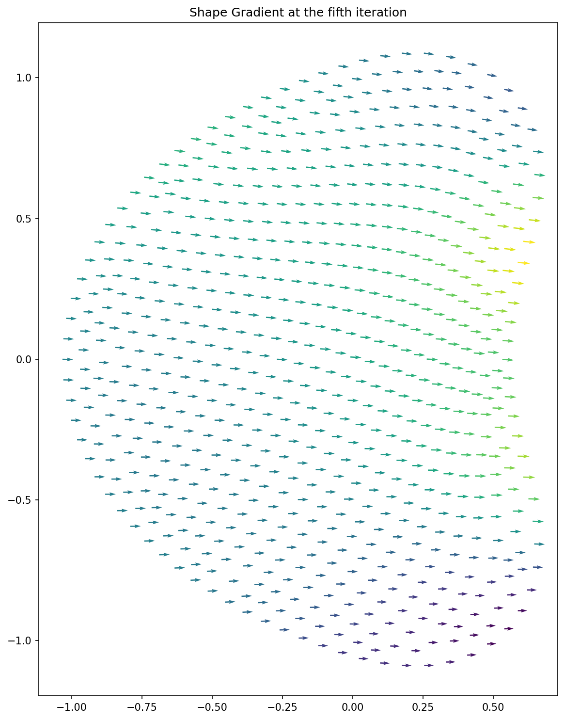
Reading vector-valued functions#

When considering vector-valued functions, we need to specify the vector dimension of the function in order to read it back into python. We demonstrate this by considering the shape gradient of the problem solved above. This can be read into python with the code

shape_gradient = cashocs.io.read_function_from_xdmf(
    "./results/checkpoints/shape_gradient.xdmf",
    "gradient_0",
    "CG",
    1,
    vector_dim=2,
    step=5,
)

Here, we load the shape gradient at the fifth iteration and visualize it with the code

plt.figure(figsize=(10, 10))
plot(shape_gradient)
plt.title("Shape Gradient at the fifth iteration")
plt.tight_layout()
# plt.savefig("./img_shape_gradient.png", dpi=150, bbox_inches="tight")

The result looks as follows