Topology Optimization with a Volume Constraint#
Problem Formulation#
In this demo, we consider topology optimization problems with a volume constraint. To demonstrate how the volume constraint is added in the implementation, we consider the already treated cantilever example from linear elasticity, which was introduced in Topology Optimization with Linear Elasticity - Cantilever. We define the topology optimization problem as
As before, \(u\) is the deformation of a linear elastic material, \(\sigma(u)\) is Hooke’s tensor. The coefficient \(\alpha_\Omega\) is given by \(\alpha_\Omega(x) = \chi_\Omega(x)\alpha_\mathrm{in} + \chi_{\Omega^c}(x) \alpha_\mathrm{out}\) and it models the elasticity of the material. In contrast to before, where we used a penalization of the used volume, we introduce an actual volume constraint here with \(V_L\) and \(V_U\) being the lower and upper volume restriction for \(\Omega\), respectively. On the Dirichlet boundary \(\Gamma_D\), the material is fixed, and at the Neumann boundary \(\Gamma_N\) a load \(g\) is applied.
Note that the generalized topological derivative for this problem does not change compared to Topology Optimization with Linear Elasticity - Cantilever and is given by
where \(r_\mathrm{in} = \frac{\alpha_\mathrm{out}}{\alpha_\mathrm{in}}\), \(r_\mathrm{out} = \frac{\alpha_\mathrm{in}}{\alpha_\mathrm{out}}\), and \(\kappa = \frac{\lambda + 3\mu}{\lambda + \mu}\). Here, \(\mu\) and \(\lambda\) are the Lamé parameters which satisfy \(\mu \geq 0\) and \(2\mu + d \lambda > 0\), where \(d\) is the dimension of the problem.
The volume constraint is treated by projecting the level-set function so that the updated level-set function satisfies the volume constraint, similar to a projected gradient method. For more details, we refer to our preprint Baeck, Blauth, Leithäuser, Pinnau, and Sturm - A Novel Deflation Approach for Topology Optimization and Application for Optimization of Bipolar Plates of Electrolysis Cells, where the used method is described detailedly.
Implementation#
The complete python code can be found in the file demo_projection.py,
and the corresponding config can be found in config.ini.
The first part of the code is completely analogous to Topology Optimization with Linear Elasticity - Cantilever and therefore we omit the details here and just state the corresponding code
from fenics import *

import cashocs

cfg = cashocs.load_config("config.ini")

mesh, subdomains, boundaries, dx, ds, dS = cashocs.regular_mesh(
    64, length_x=2.0, diagonal="crossed"
)

V = VectorFunctionSpace(mesh, "CG", 1)
CG1 = FunctionSpace(mesh, "CG", 1)
DG0 = FunctionSpace(mesh, "DG", 0)

psi = Function(CG1)
psi.vector().vec().set(1.0)
psi.vector().apply("")

E = 1.0
nu = 0.3
mu = E / (2.0 * (1.0 + nu))
lambd_star = E * nu / ((1.0 + nu) * (1.0 - 2.0 * nu))
lambd = 2 * mu * lambd_star / (lambd_star + 2.0 * mu)

alpha_in = 1.0
alpha_out = 1e-3
alpha = Function(DG0)


def eps(u):
    return Constant(0.5) * (grad(u) + grad(u).T)


def sigma(u):
    return Constant(2.0 * mu) * eps(u) + Constant(lambd) * tr(eps(u)) * Identity(2)


class Delta(UserExpression):
    def __init__(self, *args, **kwargs):
        super().__init__(*args, **kwargs)

    def eval(self, values, x):
        if near(x[0], 2.0) and near(x[1], 0.5):
            values[0] = 3.0 / mesh.hmax()
        else:
            values[0] = 0.0

    def value_shape(self):
        return ()


delta = Delta(degree=2)
g = delta * Constant((0.0, -1.0))

u = Function(V)
v = Function(V)

F = alpha * inner(sigma(u), eps(v)) * dx - dot(g, v) * ds(2)

bcs = cashocs.create_dirichlet_bcs(V, Constant((0.0, 0.0)), boundaries, 1)
Setup of the Cost Functional and Topological Derivative#
To define the topology optimization problem, we need to define the cost functional of the problem, which is similar to the cost functional in Topology Optimization with Linear Elasticity - Cantilever except the penalty term for the volume and reads
J = cashocs.IntegralFunctional(alpha * inner(sigma(u), eps(u)) * dx)
Note, that this is indeed the same as in Topology Optimization with Linear Elasticity - Cantilever for the case that
:math:\gamma = 0.
Finally, we specify the generalized topological derivative of the problem
with the lines
kappa = (lambd + 3.0 * mu) / (lambd + mu)
r_in = alpha_out / alpha_in
r_out = alpha_in / alpha_out

dJ_in = Constant(
    alpha_in * (r_in - 1.0) / (kappa * r_in + 1.0) * (kappa + 1.0) / 2.0
) * (
    Constant(2.0) * inner(sigma(u), eps(u))
    + Constant((r_in - 1.0) * (kappa - 2.0) / (kappa + 2 * r_in - 1.0))
    * tr(sigma(u))
    * tr(eps(u))
)
dJ_out = Constant(
    -alpha_out * (r_out - 1.0) / (kappa * r_out + 1.0) * (kappa + 1.0) / 2.0
) * (
    Constant(2.0) * inner(sigma(u), eps(u))
    + Constant((r_out - 1.0) * (kappa - 2.0) / (kappa + 2 * r_out - 1.0))
    * tr(sigma(u))
    * tr(eps(u))
)
This generalized topological derivative is again similar to Topology Optimization with Linear Elasticity - Cantilever
without the last term resulting from the volume penalty term in the objective, as
:math:\gamma = 0 in this demo since the volume constraint is dealt with differently.
The update routine for the level-set function reads
def update_level_set():
    cashocs.interpolate_levelset_function_to_cells(psi, alpha_in, alpha_out, alpha)
Definition and Solution of the Topology Optimization Problem#
We introduce an inequality constraint for the volume with lower border 0.5 and the upper one as 1.25
vol_low = 0.5
vol_up = 1.25
volume_restriction = (vol_low, vol_up)
Now, we are able to define the
TopologyOptimizationProblem.
top = cashocs.TopologyOptimizationProblem(
    F,
    bcs,
    J,
    u,
    v,
    psi,
    dJ_in,
    dJ_out,
    update_level_set,
    volume_restriction=volume_restriction,
    config=cfg,
)
Finally, we can solve the topology optimization problem using the
solve method.
top.solve(algorithm="bfgs", rtol=0.0, atol=0.0, angle_tol=1.0, max_iter=100)
Note
In the case of an equality constraint for the volume of \(\Omega\) we
have to use a float for volume_restriction instead of a tuple. For example, if
we consider a volume equality with target volume of 1, then we would have to use the
following definition
volume_restriction = 1.0
top = cashocs.TopologyOptimizationProblem(
   F, bcs, J, u, v, psi, dJ_in, dJ_out, update_level_set, volume_restriction=volume_restriction, config=cfg
)
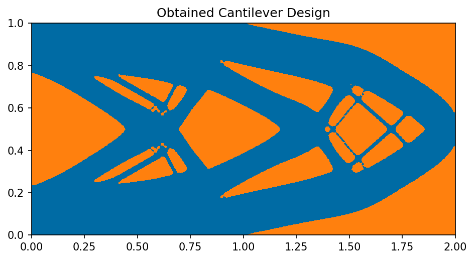
As before, we can visualize the result using the following code
import matplotlib.pyplot as plt

top.plot_shape()
plt.title("Obtained Cantilever Design")
plt.tight_layout()
# plt.savefig("./img_projection.png", dpi=150, bbox_inches="tight")
and the result looks like this