Pseudo Time Stepping for Steady State Problems#

Problem Formulation#

In this demo, we consider how to use pseudo time stepping as solver for steady state problems in the context of the shape optimization problem already considered in Optimization of an Obstacle in Stokes Flow. The problem reads

\[\begin{split} \begin{align} &\min_\Omega J(u, \Omega) = \int_{\Omega^\text{flow}} Du : Du\ \text{ d}x \\ &\text{subject to } \qquad \begin{alignedat}[t]{2} - \Delta u + \nabla p &= 0 \quad &&\text{ in } \Omega, \\ \text{div}(u) &= 0 \quad &&\text{ in } \Omega, \\ u &= u^\text{in} \quad &&\text{ on } \Gamma^\text{in}, \\ u &= 0 \quad &&\text{ on } \Gamma^\text{wall} \cup \Gamma^\text{obs}, \\ \partial_n u - p n &= 0 \quad &&\text{ on } \Gamma^\text{out}. \end{alignedat} \end{align} \end{split}\]

The corresponding regularized version of the problem including the necessary geometrical constraints are not repeated here but can be found in Optimization of an Obstacle in Stokes Flow.

Pseudo Time Stepping#

The idea behind so-called pseudo time stepping is to introduce an artificial time dependence to a steady-state problem and then using standard time stepping techniques to reach the sought steady state.

Abstractly, the method works as follows. Suppose that we want to solve a steady state PDE given by \(F(u) = 0\). For example consider the problem

\[ F(u) = -\Delta u - f, \]

which corresponds to Poisson’s equation, i.e.,

\[ -\Delta u = 1. \]

For linear problems, pseudo time stepping is usually not required, so that we could also consider the nonlinear problem

\[ F(u) = -\Delta u + u^3 - 1. \]

Introducing a pseudo time, which we denote by \(\tau\), the instationary equation would be of the form

\[ \frac{\partial u}{\partial \tau} + F(u) = 0. \]

This would correspond to the following PDE:

\[ \partial_\tau u -\Delta u + u^3 = 1 \]

in our second example.

Obviously, if the equation has a steady-state solution, we can try to approximate it by solving the (pseudo) instationary one until \(\tau \to \infty\), or until the steady state is reached. For this reason, time stepping schemes, such as the explicit or implicit Euler method, the Crank Nicolson scheme, Runge-Kutta methods or Backwards-Differentiation-Formula can be applied. Not all of them are suited for obtaining a steady state solution. Explicit schemes are cheap to compute, but do not exhibit the necessary stability properties. Best suited are implicit methods, particularly the implicit or backwards Euler method as they tend to damp the solution into the steady state.

Note

One can easily verify that using the implicit Euler method with a stepsize of \(\Delta \tau = \infty\) corresponds to the classical Newton method for solving \(F(u) = 0\). Hence, pseudo time stepping can be seen as a relaxation or globalization of Newton’s method.

In our case, the instationary Stokes system is given by

\[\begin{split} \begin{alignedat}{2} \partial_\tau u - \Delta u + \nabla p &= 0 \quad &&\text{ in } \Omega,\\ \text{div}(u) &= 0 \quad &&\text{ in } \Omega, \end{alignedat} \end{split}\]

supplemented with the previously defined boundary conditions. Note that, due to the incompressibility constraint, there is no (pseudo) time derivative of the pressure so that this component later on has to be excluded from the time derivative. In the following, we will discuss how to use pseudo time stepping with cashocs.

Implementation#

The complete python code can be found in the file demo_pseudo_time_stepping.py, and the corresponding config can be found in config.ini.

Definition of state equation and cost functional#

Most of the code listed here is completely identical to the one presented in Optimization of an Obstacle in Stokes Flow so that we do not go over this detailedly. The following code defines the state equation and cost functional, and the changes begin just before the definition of the shape optimization problem.

from fenics import *

import cashocs

config = cashocs.load_config("./config.ini")
mesh, subdomains, boundaries, dx, ds, dS = cashocs.import_mesh("./mesh/mesh.xdmf")

v_elem = VectorElement("CG", mesh.ufl_cell(), 2)
p_elem = FiniteElement("CG", mesh.ufl_cell(), 1)
V = FunctionSpace(mesh, MixedElement([v_elem, p_elem]))

up = Function(V)
u, p = split(up)
vq = Function(V)
v, q = split(vq)

e = inner(grad(u), grad(v)) * dx - p * div(v) * dx - q * div(u) * dx

u_in = Expression(("-1.0/4.0*(x[1] - 2.0)*(x[1] + 2.0)", "0.0"), degree=2)
bc_in = DirichletBC(V.sub(0), u_in, boundaries, 1)

bc_no_slip = cashocs.create_dirichlet_bcs(
    V.sub(0), Constant((0, 0)), boundaries, [2, 4]
)
bcs = [bc_in] + bc_no_slip

J = cashocs.IntegralFunctional(inner(grad(u), grad(u)) * dx)

Setting up the pseudo time stepping#

Now, we come to the interesting part, namely how to use pseudo time stepping with cashocs. It is really easy, as only the options for the PETSc solver have to be modified. Cashocs notices this and changes to the pseudo time stepping solver in an appropriate fashion. For a detailed introduction to the usage of the PETSc options, we refer the reader to Iterative Solvers for State and Adjoint Systems. For this problem, we use the following options for PETSc:

petsc_options = {
    "ts_type": "beuler",
    "ts_max_steps": 100,
    "ts_dt": 1e0,
    "snes_type": "ksponly",
    "snes_rtol": 1e-6,
    "snes_atol": 1e-10,
    "ksp_type": "preonly",
    "pc_type": "lu",
    "pc_factor_mat_solver_type": "mumps",
}

Here, we specify that the implicit / backwards Euler method shall be used as time stepping scheme with the option "ts_type": "beuler". Additionally, we have to specify the maximum amount of pseudo time stepping iterations with "ts_max_steps" and specify the time step size with "ts_dt". Here, the time step size is not critical, as we solve the linear Stokes system, but for other equations the time step may be restricted, e.g., by some CFL-type condition. To ensure that in each time step only a single linear system is used, the option "snes_type": "ksponly" is used. It is usually more efficient to only do a single iteration of the nonlinearity per pseudo time step, leading to a linearly implicit Euler method. However, here all possibles PETSc SNES options can be set.

Moreover, the relative and absolute tolerances (based on the residual of \(F(u) = 0\)) for the pseudo time stepping are defined with "snes_rtol": "1e-6" and "snes_atol": "1e-10". Hence, these parameters specify two things: First, the tolerances for the SNES for each pseudo time step. Here, this is not active as we have chosen the “ksponly”, but, e.g., for "snes_type": "newtonls" the tolerances would be active. Second, the parameters also specify the tolerances for the convergence of the pseudo time stepping method, based on the residual of the actual nonlinear equation. However, as it does not make much sense to use a different tolerance for these two things, this doubling of parameters should be fine for most applications. We would usually recommend to use "snes_type": "ksponly" anyway, as this only does a single iteration of Newton’s method per pseudo time step and this is usually sufficient anyway.

Finally, the options for the linear solver are specified analogously to the discussion in Iterative Solvers for State and Adjoint Systems.

Additionally, to make the solver behavior more verbose, we enable the debug logger of cashocs with the line

cashocs.set_log_level(cashocs.log.DEBUG)

Finally, the shape optimization problem can be set up and solved as has been done many times before. The major difference to the previous approaches are twofold. First, of course, the PETSc options have to be supplied, as in Iterative Solvers for State and Adjoint Systems. Second, we exclude the pressure component of the mixed finite element formulation for the Stokes system via the keyword argument excluded_from_time_derivative=[1]. This ensures that the second component with index 1 (in python) is excluded from the time derivative - which is just what we wanted as explained in the discussion in the beginning.

sop = cashocs.ShapeOptimizationProblem(
    e,
    bcs,
    J,
    up,
    vq,
    boundaries,
    config=config,
    ksp_options=petsc_options,
    excluded_from_time_derivative=[1],
)
sop.solve()

Attention

In order to use the pseudo time stepping, users have to change the backend for the state system to use PETSc. This is done with the lines

config.ini#

[StateSystem]
is_linear = False
backend = petsc

Here, we additionally have to use is_linear = False to use the pseudo time stepping - but of course this setting also works for linear problems.

From the debug log we can nicely see that cashocs is indeed using pseudo time stepping to solve the state and adjoint systems. Additionally, as we have a linear equation and a rather large time step size, the pseudo time stepping approach converges really fast, only requiring about 5 pseudo time steps.

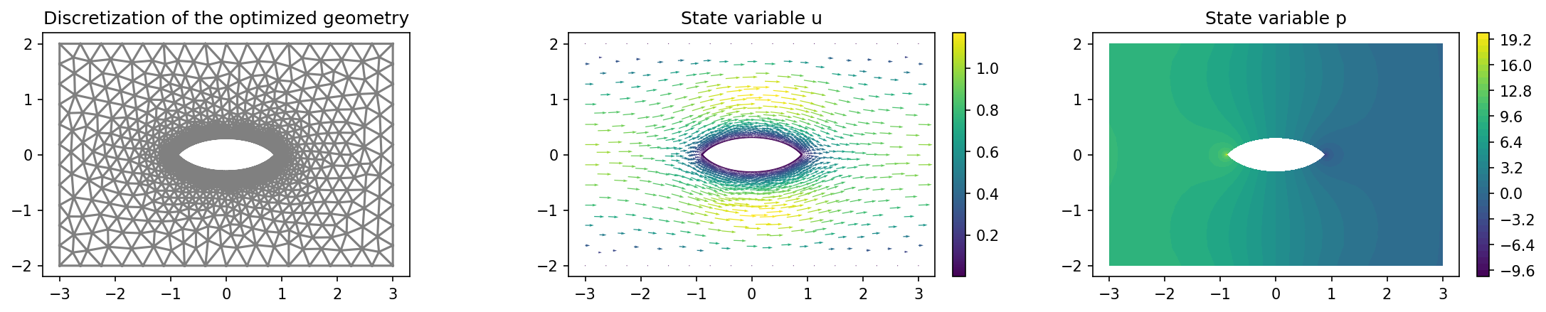
Finally, the optimized geometry looks as the one obtained in Optimization of an Obstacle in Stokes Flow:

import matplotlib.pyplot as plt

plt.figure(figsize=(15, 3))

ax_mesh = plt.subplot(1, 3, 1)
fig_mesh = plot(mesh)
plt.title("Discretization of the optimized geometry")

ax_u = plt.subplot(1, 3, 2)
ax_u.set_xlim(ax_mesh.get_xlim())
ax_u.set_ylim(ax_mesh.get_ylim())
fig_u = plot(u)
plt.colorbar(fig_u, fraction=0.046, pad=0.04)
plt.title("State variable u")


ax_p = plt.subplot(1, 3, 3)
ax_p.set_xlim(ax_mesh.get_xlim())
ax_p.set_ylim(ax_mesh.get_ylim())
fig_p = plot(p)
plt.colorbar(fig_p, fraction=0.046, pad=0.04)
plt.title("State variable p")

plt.tight_layout()
# plt.savefig("./img_pseudo_time_stepping.png", dpi=150, bbox_inches="tight")

and the result is shown below

../../../../_images/img_pseudo_time_stepping.png